1. Introduction

Very low earth orbit (VLEO) is an orbit with a nominal altitude of about 450 km or less, which is much lower than the conventional low earth orbit (LEO) with an altitude of 600–1200 km and the geostationary earth orbit (GEO) with an altitude of 35,768 km [1]. Compared to higher orbits, VLEO spacecraft have lower launch costs, better radiometric performance, and better resolution of optical payloads [2]. With the effect of dense atmosphere, space debris in VLEO experiences a more rapid decay rate. Compared to higher altitudes, spacecraft in VLEO are subject to less impact from space debris.

VLEO spacecraft possess unique advantages in ground observation, emergency communication, and geophysical scientific exploration, attracting interest from both national and commercial entities [3]. To facilitate material supply and reduce the threat of space debris, both the International Space Station and Chinese Space Station are located at orbital altitudes below 450 km [4, 5]. ESA’s first Core Earth Explorer mission, GOCE, is aimed at measuring the precise gravity gradient at an altitude of 250 km [6]. The US Naval Research Laboratory has launched two spherical satellites, ANDE Pollux and ANDE Castor, to improve the accuracy of LEO spacecraft orbit prediction by detecting the overall atmospheric density at an altitude of 400 km [7]. JAXA launched the Super Low Altitude Orbit Test Satellite in 2017 to test high-resolution satellite images within an altitude range of 160–270 km [8]. Commercial aerospace companies operating giant constellations, such as Starlink, also consider VLEO as the next expansion direction.

Despite the advantages of VLEO spacecraft, the challenges they encounter are evident: Atmospheric drag will significantly shorten their lifetime [9]. Large-scale spacecraft, such as the Space Station, require frequent orbital altitude boosts to meet mission requirements. Fuel for the space station can be replenished regularly, while other spacecraft often use high specific impulse propulsion technology to extend their service time. When fuel equals life, precise orbit decay prediction (PODP) becomes an important prerequisite for long-term on-orbit service. PODP provides a reliable reference for maneuvering strategies for orbit maintenance, proving to be an effective method for enhancing fuel efficiency.

PODP faces a series of challenges in practical situations. The traditional orbital prediction methods (TOPMs) based on physical models are inaccurate with divergent errors in PODP due to the challenges of modeling the atmosphere and acquiring the physical information of specific spacecraft [10]. Orbit decay with TOPM also depends on the information of space environment, which is hard to accurately predict. In recent years, several methods with machine learning techniques (MLTs) have emerged to enhance the capabilities of TOPM. Cimmino, Opromolla, and Fasano [11] used MLT to determine the ballistic coefficients of LEO spacecraft based on orbital data. This approach can minimize prediction errors stemming from uncertainties in drag coefficients and area-to-mass ratios. Lei and Zhang [12] employed another form of proximal policy optimization, PPO2, to adjust atmosphere model parameters to improve TOPM. Compared to standard orbital data, the proposed method resulted in a maximum absolute space position error of 8133.329 m on the CSS in 3 days. Peng and Bai [13] used an artificial neural network (NN) to compensate for TOPM errors. Compared to the high-precision orbital propagator (HPOP), the proposed approach significantly reduced residual errors. Li et al. [14] captured the error patterns to adjust the physical model with MLT based on historical prediction errors of space debris, which enhanced the capability of space situational awareness. Bizalion et al. [15] used MLT to derive the underlying patterns of historical error from two-line element (TLE) data, which was successful in generating valuable covariance information for a significant portion of the TLE directory.

In addition to indirectly improving TOPM with MLT, only a limited number of studies have concerned model-agnostic orbit prediction technology. Thammawichai and Luangwilai [16] proposed the nonlinear programming model to generate orbital elements based on publicly available TLE data. Relative to the SGP4 model, the proposed approach performed better. Luo, Ren, and Zhao [17] used an LSTM-CNN model and trained it with TLE data of LEO spacecraft, which resulted in an overall position error of about 200 km after 20 days.

Excluding considerations of physical models, the utilization of PODP in combination with model-agnostic MLT offers enhanced flexibility and requires lower computational resources and memory usage compared to TOPM. Furthermore, it mitigates the inherent structural bias associated with physical models and is well suited for scenarios characterized by abundant data availability. The dynamic factors influencing the decay, such as the space environment and spacecraft physical parameters, pose a challenge of catastrophic forgetting [18] for conventional MLT. Current model-agnostic MLTs face limitations in terms of their generalization capabilities. Various strategies have been extensively explored to enhance the generalization performance of NNs [19], including optimization-based methods (like meta-learning [20]), replay-based techniques (such as experience replay [21]), and regularization-based approaches (like elastic weight consolidation [EWC] [22]). Meta-learning seeks to achieve “learning to learn,” allowing NN to be flexible and adaptable in various scenarios, which has been utilized in the field of spacecraft terminal autonomous navigation and control [23–25]. Experience replay involves the creation of a small memory buffer to retain samples from previous tasks, allowing the NN to retain learned skills. This technique has been explored in spacecraft collision avoidance [26] and integrated scheduling [27]. The EWC combines historical and recent training data to update the NN parameters by applying a penalty function, commonly used to process large datasets by decomposing them into several subsets in the field of earth observation [28]. Meta-learning methods excel in few-shot learning, and experience replay efficiently constructs and utilizes memory buffers with a limited sample size. EWC is particularly suited for regression problems with abundant training data.

In this paper, the expandable orbit decay propagator (EODP) is proposed to achieve PODP of VLEO spacecraft based on model-agnostic MLT. EODP employs a deep NN (DNN) as the fundamental learner to comprehend the decaying rule and incorporates the theory of EWC. Compared to the previous method, EODP greatly improves prediction accuracy and generalization performance. Furthermore, it presents a novel approach for the future implementation of machine learning–based methods in the field of orbit prediction.

The remainder of the paper is organized as follows. First, a definition of training and testing set and an overview of the proposed EODP are provided. The plasticity of EODP is then analyzed, and the effects on the training process with different training methods are discussed. Compared to orbital data in real situations, the performance of EODP is analyzed. The results show that EODP achieves high accuracy in PODP of VLEO spacecraft and maintains excellent generalization when dealing with different spacecraft.

2. Methods

2.1. Generation of Orbital Decay Training Set

HPOP was adapted to generate the training set of VLEO spacecraft, and the effects of perturbations considered are shown in Table 1.

Table 1. Perturbation factors considered in the HPOP model.

Perturbation	Model	Detail
Nonspherical earth gravity	EGM2008 gravity model	20 × 20 harmonics
Atmospheric drag	NRLMSISE 2000 atmospheric model	—
Solar radiation pressure	Spherical solar radiation pressure model	—
Three-body attraction	“Sun, moon, and earth” gravity model	—

With the influence of the factors above, the state of spacecraft can be expressed as

$$ ()

where $$ are the vectors of acceleration and position in the J2000 coordinate system, μ is the earth gravitational constant, r is the geocentric distance, and a_E, a_D, a_R, a_tr are the perturbation accelerations caused by the nonspherical earth gravity, atmospheric drag, solar radiation pressure, and three-body attraction, respectively.

Decaying rules of VLEO spacecraft are difficult to capture directly with osculating orbital elements, while using mean orbital elements is appropriate [29].

$$ ()

$$ ()

where H(t) is the orbital altitude at time instant t; $$ is the initial altitude; $$ indicates initial mean orbit semimajor axis; R is the average equatorial radius of the earth; and a_s1, a_l2, and a_s2 are the first-order short-period factor, second-order long-period factor, and second-order short-period factor of the semimajor axis, respectively. Caused by the nonspherical earth gravity, the periodic terms of semimajor axis are associated with inclination [30], which can be described as

$$ ()

$$ ()

$$ ()

where J₂ is the EGM2008 zonal spherical harmonic coefficient of the gravitational potential to Degree 2. The a, i, f, e, and ω are the osculating orbital elements of semimajor axis, inclination, true anomaly, eccentricity, and argument of periapsis, respectively.

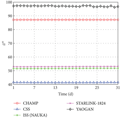
Nonspherical perturbation of the earth results in periodic alterations of a, i, and e. The primary factor contributing to decay is atmospheric drag, which does not affect i [31], as shown in Figure 1. Inclinations exhibit notable variations across different spacecraft, thereby influencing the decay rule distinctly. For deriving decay rule at various i, the generation of the training data should account for the variability of i.

The calculation error of atmospheric drag is the main issue that affects the accuracy of TOPM [32]. The atmospheric drag acceleration can be expressed as

$$ ()

where a_D is the acceleration caused by atmospheric drag, C_d is the drag coefficients, S and M are the effective resistance area and mass, respectively, ρ stands for atmospheric density at the current position, v is the velocity relative to airflow, and $$ is the unit vector of v.

Spacecraft usually lose the ability of attitude control during decay, which directly affects the effective drag area. Due to the complexity and variability of the atmosphere environment and attitude of the spacecraft, factors such as the angle of airflow, material properties of spacecraft surfaces, and atmospheric humidity will affect C_d. Accurate values of C_d and S/M are difficult to figure out when considering the above factors. To avoid the negative effect caused by determination errors of C_d and S/M, the generation of the training set should consider the variation of them.

Accurate modeling methods for the atmosphere have always been a concern. A series of achievements have been proposed, including the Harris–Priester model, which considers weekly variations. Additionally, the three-dimensional atmospheric models DTM2012 and NRLMSIS 2000 take altitude, season, latitude, and weekly variations into account. Bowman et al. [33] introduced new exospheric temperature equations, semiannual density equations, and geomagnetic storm equations, which significantly reduce the density errors during major geomagnetic storm periods. The accuracy of atmospheric models is limited by the information of space weather, especially solar activity (F10.7) and geomagnetism (K_p) [34]. Characterizing atmospheric density with these two factors is reasonable and practicable. To avoid the negative effect caused by determination errors of atmospheric density, the generation of the training set should also consider the variations of F10.7 and K_p.

In summary, the training set contains compositional information of six dimensions, and one sample can be represented as follows:

$$ ()

McCreary [35] put forward a series of recommendations for missions in VLEO, proposing the establishment of a circular sun-synchronous orbit with a semimajor axis of 6608 ± 70 km. With reference to their suggestions, this study focuses on the VLEO spacecraft with circular or nearly circular orbits. The parameters of H and i are defined within the intervals of [150 km, 300 km] and [90°, 110°], respectively.

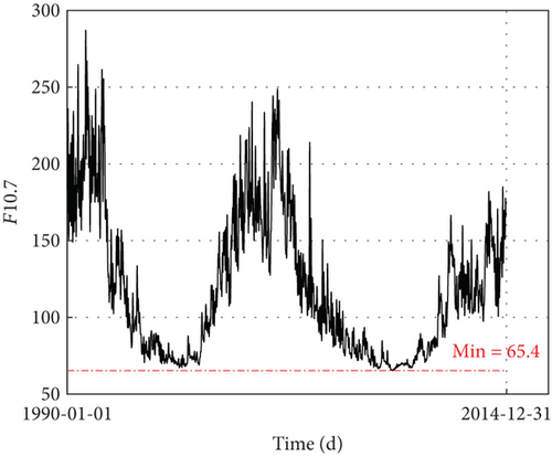
Observation data of F10.7 from 1990-01-01 to 2014-12-31 is shown in Figure 2. The data is sourced from the CelesTrak website. F10.7 usually falls within the range of [65, 300]. In this study, F10.7 is set within the range of 70–280 due to the low likelihood of extreme values.

The K_p typically uses 28 values to qualify the strength of geomagnetic activity [36], which can be described as

$$ ()

For C_d and S/M, there are no standardized criteria, which can be set as follows:

$$ ()

where S/M stands for the area-to-mass ratios. In a word, all elements of the training set are shown in Table 2.

Table 2. The range of every element of training set.

Symbol	Element	Type	Range
Kp	Geomagnetic index	Discrete	[0, 27]
F10.7	Solar activity	Discrete	[70, 280]
H	Altitude (km)	Continuous	[150, 300]
i	Inclination (°)	Discrete	[90, 110]
Cd	Drag coefficient	Discrete	[2.2, 2.8]
S/M	Area-to-mass ratios (m2/kg)	Discrete	[0.005, 0.02]

The structure of the training set is illustrated in Figure 3, where t₀ and t_end indicate the beginning and the end of the orbit epoch. Each sample consists of continuous data (time series vector of H) and discrete data (other elements). Time series data is generated by HPOP with specific values of K_p, F10.7, i, C_d, S/M, and $$. The sampling interval is set to 1 h.

The values of K_p, F10.7, i, C_d, and S/M are set as follows.

$$ ()

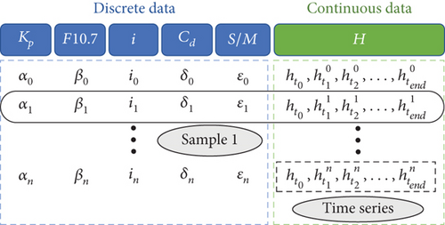
A total of 216,720 samples are generated. With different values of K_p, F10.7, i, C_d, S/M, and $$, the length of the time series in each sample may be different.

2.2. Description of Orbital Decay Testing Set

The testing set is crucial for evaluating MLT performance. In this study, VLEO spacecraft with precise location and no maneuvering effects is the ideal test object. The model should fit well to the testing data produced by HPOP. Additionally, more realistic orbital data should be utilized. Data involved in the testing set consists of the following two parts:

• a.

  The CPF ephemeris files from the International Laser Ranging Service (ILRS).

• b.

  The data generated by HPOP.

CPF ephemeris is a high-precision forecast data derived from the advancement of satellite laser ranging technology [37]. CPF files are available from Crustal Dynamics Data Information System (CDDIS) or EUROLAS Data Center (EDC). CPF data is more precise during short-term forecasting than TLE and more credible due to continuous tracking and monitoring. The CPF data has a prediction error of less than 1 m for LEO spherical satellites and approximately 100 m for LEO nonspherical satellites, which can serve as a reference for the actual position of VLEO spacecraft. ILRS collects a portion of resident space object observation data, and the corresponding CPF data are provided by 29 institutes.

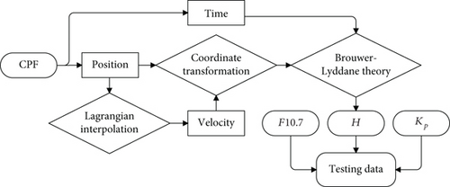
The CPF data contains information about the orbital epoch, sampling time, and position data in the earth-fixed coordinate system. With the process shown in Figure 4, the CPF data can be converted to testing set, mainly including H, K_p, and F10.7, at the corresponding time. Orbital epoch, sampling time, and corresponding position data in CPF are first extracted and processed according to a standard format. Then, the 10th-order Lagrangian interpolation is applied to estimate the velocity information. With the Brouwer–Lyddane theory [38], which also can be described as Equation (2), processed data can be converted to H. The corresponding K_p and F10.7 are obtained from CelesTrak.

2.3. Description of EODP

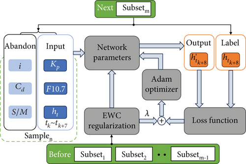
The proposed method, EODP, is an extensible application of DNN on PODP based on EWC, which is utilized to address the issue of catastrophic forgetting in MLT. The theory of EWC posits that knowledge or rules acquired during training are stored in the parameters (weights and bias) of NN. The primary approach of EWC to maintain memory in a dynamic environment involves the identification of critical parameters and the implementation of a penalty function to constrain their significant alteration during subsequent training.

H is the main object of concern, serving as both input and output. The orbit epoch of each sample is the primary factor influencing the extent of data redundancy. A sufficiently long-period epoch will bring a large amount of redundant data and easily lead to overfitting. In this study, training set is divided into several subsets based on the initial altitude, such as $$, and the orbit epoch of each sample is limited to 3 days. Different training subsets stand for different rules of decay.

Training a model with all parameters obviously increases the computational complexity and the possibility of overfitting. The i, C_d, and S/M do not serve as the key factors influencing the training of NN, which are not considered as the inputs. When training with Sample_n at time t_k, a time series consisting of K_p, F10.7, and h_t in [t_k, t_k+Δk] is required as input. The time series will be labeled as $$. In this study, Δk is set to 7. The input of historical observations (a time series) enables EODP to predict the future situation of decay accurately. From another perspective, historical observations implicitly contain the information of i,  C_d, and S/M, which can help avoid the challenge in determining the physical parameters of specific spacecraft and correct errors introduced by the atmospheric model to some extent.

Figure 5 illustrates the process of the m-th training with Sample_n. To capture the rule of Subset_m, EWC regularization needs to be computed using the previous m − 1 subsets.

The computation of m-th EWC regularization (L_m) is related to the network parameters of last training, which can be described as

$$ ()

where the matrix θ_now and $$ indicate current and previous network parameters (weights and bias), respectively, λ_m stands for the m-th significant coefficient of learned knowledge from m − 1 subsets, and F_m represents the m-th weight matrix of all network parameters, which is a diagonal matrix. Elements of F_m come from the average gradient variation of network parameters, which are described as follows:

$$ ()

where f_nn is the n-th diagonal element of F_m, A represents the previously used training subsets, N is the number of samples in Subset_m, $$ is the n-th network parameter of $$, and a_j is the j-th sample of A.

3. Feature Analysis of EODP

3.1. Plasticity of Network Parameters

EODP extends the ability to master the rules from different training subsets by modulating the plasticity of network parameters. The plasticity of network parameters is a fundamental feature of NN, which is manifested in two perspectives. (1) The NN trained with the current subset can be applied in other scenarios. (2) NN exhibits varying performance in different regions due to differing densities of the same training subset. The architecture of NN is shown in Table 3.

Table 3. The architecture of NN.

Name	Description	Definition
Optimizer	Learning algorithm	Adam
Neurons of hidden layer	Layer 1	6
	Layer 2	16
	Layer 3	16
	Layer 4	6
Activation function	Between Layer 1 and Layer 2	ReLU
	Between Layer 2 and Layer 3	ReLU
	Between Layer 3 and Layer 4	ReLU
Learning rate	—	0.005

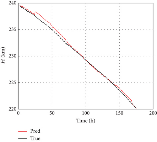
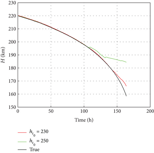
The model trained with the subset of $$ is also applicable to the altitude of 240–220 km, illustrating the first aspect of plasticity, as depicted in Figure 6.

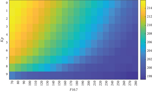
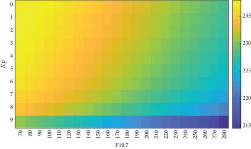
As the heatmaps shown in Figures 7(a) and 7(b), the data distribution in the training subset₁ ($$) and subset₂ ($$) is different. Data in subset₁ is more concentrated at altitudes of less than 200 km, while data in subset₂ is completely opposite. The performance of NN trained with subset₁ is better than that trained with subset₂ at the altitudes around 200 km, which reflects the second perspective.

3.2. Application of Plasticity in Training Strategies

Plasticity plays a crucial role in the training strategies of EODP, involving the utilization of different combinations of training subsets. With a reasonable size of training set, the achievement of exceptional performance is enabled. When analyzing the decay at altitudes ranging from 150 to 300 km, various combinations of training subsets are outlined in Table 4. Testing data is generated by HPOP, with an initial altitude of 280 km and an orbit epoch of around 50 days.

Table 4. Different training strategies.

Strategies	Set 1	Set 2	Set 3	Set 4
$$ (km)	[210, 230, 250, 270, 290]	[210, 250, 290]	[230, 290]	[290, 230]

EODP is subjected to various training strategies as outlined in Table 4, and its performance is illustrated in Figure 8. EODP, when trained with each dataset, consistently demonstrates exceptional performance throughout the entire orbit epoch of the test data. The analysis of absolute errors in Figure 8(b) reveals that EODP, when trained with extensive data (such as Set 1 and Set 2), exhibits more stable and accurate performance. Towards the end of the orbit epoch, there is a notable spike in errors, which is attributed to the limited time interval for sample generation. The narrow epoch interval results in sparse data at lower altitudes, leading to a marginal decline in prediction accuracy. This scenario is particularly pronounced in models trained with Set 3 and Set 4.

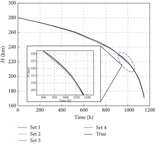
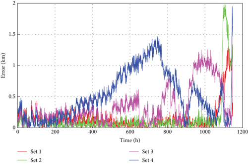
The performance depicted in Figure 8 is assessed using statistical metrics, including root mean squared error (RMSE, primarily considered), median absolute error, and mean absolute error. As illustrated in Table 5, the performance of the EODP trained with Set 1 and Set 2 surpasses that of Set 3 and Set 4, suggesting that a more extensive training data leads to enhanced overall prediction accuracy. In certain instances, obtaining λ becomes challenging with a large number of training subsets, which will easily result in heightened prediction volatility. The training approach becomes more adaptable due to the plasticity effect. In comparison to Set 1, the performance of the model trained with Set 2 is considered satisfactory in certain instances, indicating the potential for regulating the size of the training set.

Table 5. Evaluation of the performance of EODP trained with different strategies.

Strategies	RMSE (km)	Mean absolute error (km)	Median absolute error (km)
Set 1	0.2644	0.1677	0.1143
Set 2	0.3865	0.1678	0.0720
Set 3	0.7158	0.3999	0.2499
Set 4	0.8417	0.5564	0.4385

4. Results on Real Case

The performance of EODP, trained with Set 1, is analyzed in real-world scenarios. To avoid the negative effects of maneuvers, spacecraft at the end of their lifetime are suitable as test objects, such as CHAMP and ANDE Pollux. Table 6 illustrates the initial states of the two spacecraft at specific orbit epochs. The $$ can be inverted from CPF data. C_d and S/M are estimated from official technical documents [7]. Testing data from HPOP is generated based on the same state. F10.7 and K_p are derived from the observational data, which is sampled once a day.

The performance on actual cases of CHAMP and ANDE Pollux with the EODP is illustrated in Figures 9 and 10. The EODP shows outstanding performance on testing data created by HPOP, with a maximum absolute error of around 0.3 km. With a maximum absolute error of less than 1 km in 136 h, EODP also achieves PODP on real VLEO spacecraft. When analyzing the same spacecraft, the performance of EODP varies at different altitudes. The increasing prediction error in some cases is caused by data sparsity at low altitudes and inappropriate values of λ that leads to a marginal decline in prediction accuracy. Different values of λ for distinct training subsets indicate varying levels of focus on these rules, leading to different performance in various situations.

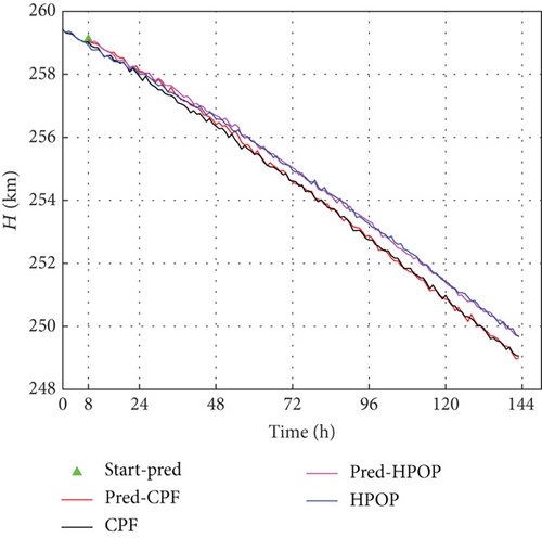
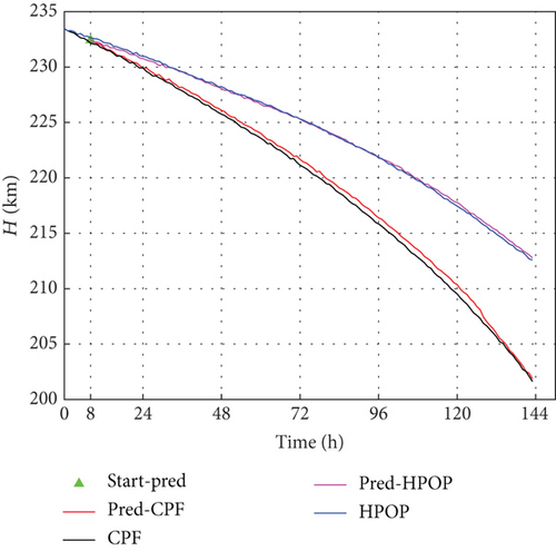
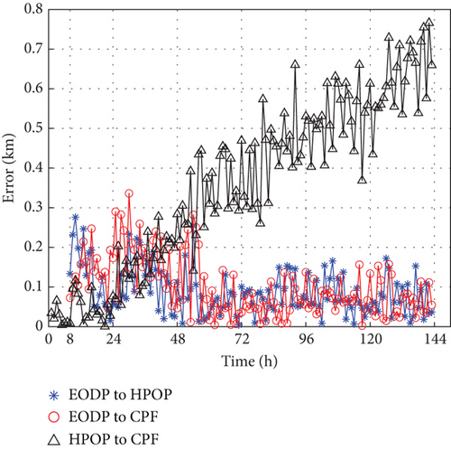
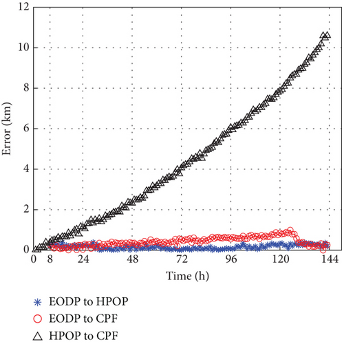
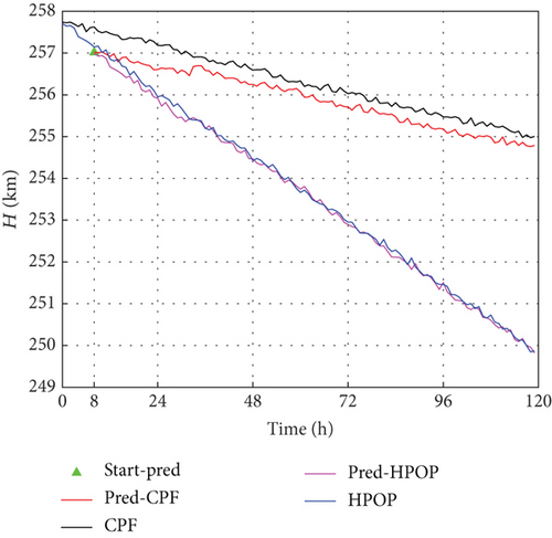
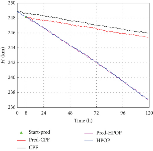
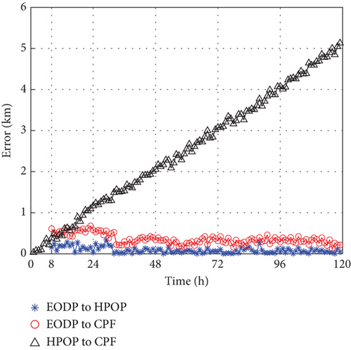
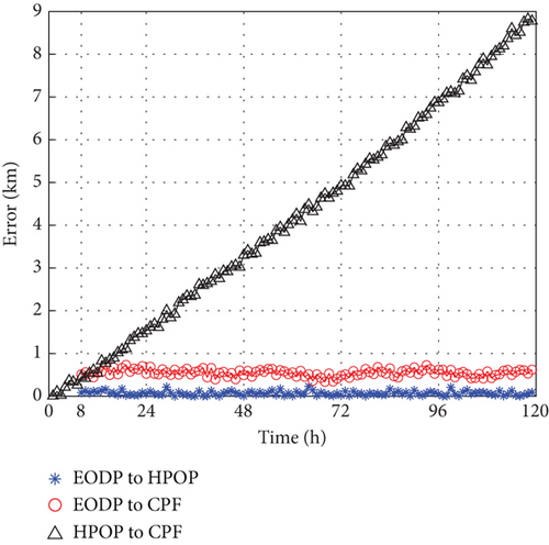
A significant disparity between HPOP data and CPF data is mainly due to the inherent limitations of TOPM, uncertainties in physical parameters, and future space environment, leading to deteriorating performance. For specific spacecraft with a spherical shell and stable surface materials (such as ANDE Pollux), TOPM can perform well in PODP. In fact, the C_d and S/M of the CHAMP vary during decaying, which leads to critical error prediction. Due to the lack of equivalent accuracy in the parameters, the error of the testing data generated by HPOP relative to CPF is quite different. In this study, the proposed method, EODP, effectively overcomes the challenge of estimating physical parameters and achieves higher accuracy in PODP.

RMSE, median error, and mean error are used to evaluate the performance of EODP on actual cases, as shown in Tables 7, 8, and 9. EODP can be applied to various scenarios. Compared to HPOP for lower altitude cases, the accuracy is enhanced by approximately 90%, such as the second orbit epoch of ANDE Pollux (5 days) and CHAMP (6 days). For higher altitudes, the prediction accuracy is improved by at least 70%.

5. Conclusion

In this paper, the proposed method of EODP for implementing PODP based on historical data demonstrates high accuracy. EODP leverages the EWC, a method of continual learning, and addresses the limited generalization ability. This results in improved performance on PODP for various spacecraft and enhances the applicability of MLT in orbit prediction. EODP also overcomes the challenge of inaccurate physical parameter and future space environment estimation. Meanwhile, the EODP can be further extended by adjusting the initial altitude and important coefficients of different training subsets. This implies that the EODP can be utilized for PODP covering all LEO and VLEO spacecraft, including space debris. With EODP, powerful data support is easily provided for orbit maintenance and high-precision flight control of spacecraft.

Conflicts of Interest

The authors declare no conflicts of interest.

Funding

This research is supported by the National Science Fund for Distinguished Young Scholars (doi: 10.13039/501100014219) (12125207) and National Natural Science Foundation of China (doi: 10.13039/501100001809) (12372052). The authors are grateful for the financial support from Technology Innovation Team of Manned Space Engineering.