Volume 2024, Issue 1 8843680

Research Article

Open Access

Modeling and Analysis of Fasciola Hepatica Disease Transmission

Dagnaw Tantie Yihunie,

Corresponding Author

Dagnaw Tantie Yihunie

[email protected]

orcid.org/0000-0003-1800-3499

Department of Mathematics , Bahir Dar University , P.O. Box 79 , Bahir Dar , Ethiopia , bdu.edu.et

Search for more papers by this author

Joseph Y. T. Mugisha,

Joseph Y. T. Mugisha

Department of Mathematics , Makerere University , P.O. Box 7062 , Kampala , Uganda , mak.ac.ug

Search for more papers by this author

Dawit Melese Gebru,

Dawit Melese Gebru

Department of Mathematics , Bahir Dar University , P.O. Box 79 , Bahir Dar , Ethiopia , bdu.edu.et

Search for more papers by this author

Haileyesus Tessema Alemneh,

Haileyesus Tessema Alemneh

Department of Mathematics , University of Gondar , P.O. Box 196 , Gondar , Ethiopia , uog.edu.et

Search for more papers by this author

Dagnaw Tantie Yihunie,

Corresponding Author

Dagnaw Tantie Yihunie

[email protected]

orcid.org/0000-0003-1800-3499

Department of Mathematics , Bahir Dar University , P.O. Box 79 , Bahir Dar , Ethiopia , bdu.edu.et

Search for more papers by this author

Joseph Y. T. Mugisha,

Joseph Y. T. Mugisha

Department of Mathematics , Makerere University , P.O. Box 7062 , Kampala , Uganda , mak.ac.ug

Search for more papers by this author

Dawit Melese Gebru,

Dawit Melese Gebru

Department of Mathematics , Bahir Dar University , P.O. Box 79 , Bahir Dar , Ethiopia , bdu.edu.et

Search for more papers by this author

Haileyesus Tessema Alemneh,

Haileyesus Tessema Alemneh

Department of Mathematics , University of Gondar , P.O. Box 196 , Gondar , Ethiopia , uog.edu.et

Search for more papers by this author

First published: 17 July 2024

https://doi.org/10.1155/2024/8843680

Academic Editor: Alberto Fiorenza

Share a link

Email
Wechat
Bluesky

Abstract

In this paper, a mathematical model for the transmission dynamics of Fasciola hepatica in cattle and snail populations is formulated and analyzed. The snail mortality rate (μ_s) is the most important factor that indirectly impacts the basic reproduction number (R₀). A 50% change, either an increase or decrease, in the snail mortality rate will result in an approximate 50% change in the opposite direction in the value of R₀. The model shows a forward bifurcation at R₀ = 1, indicating that the disease dynamics undergo a critical transition at this threshold. This change signifies a transition from a disease-free state to a persistent infection, highlighting the possibility of a continuous disease presence given specific epidemiological conditions. Simulations show that reducing miracidia, metacercariae, and snail populations, improving treatment, and lowering pathogen transfer between cattle and snails significantly decrease disease prevalence in cattle. To control the disease, transmission rates for cattle and snails must be reduced below γ_c = 1.4338 × 10⁻⁷ and γ_s = 1.1473 × 10⁻⁸, respectively. Current treatments are insufficient, and a combination of improved treatments reduced transmission rates, and increased snail mortality is recommended for better disease control.

1. Introduction

Fasciololasis (known as “liver fluke”) is a zoonotic disease induced by two parasitic flatworms or trematodes called fasciola gigantica and fasciola hepatica, which primarily affect the liver [1, 2]. The World Health Organization (WHO) has prioritized it as a neglected tropical disease that can affect both humans and livestock [3, 4]. It is a worldwide disease that primarily affects domesticated pets like cattle, goats, and sheep, but it can also affect humans [5]. Animal fascioliasis is a major issue that has a global impact on livestock productivity [6] and a serious problem in the veterinary field all over the world [7]. The fasciola parasite is observed in the livers of infected remnants as well as the bile ducts. Fasciololasis is a waterborne and foodborne zoonosis that is commonly acquired by drinking and eating the parasite metacercaria that is encysted in water and food [1].

Fascioliasis is becoming more common worldwide, and there is a strong correlation with a high infection rate among ruminant definitive hosts. Except for Antarctica, fascioliasis is endemic worldwide [8]. Fasciola hepatica is found worldwide but is most common in temperate areas, whereas Fasciola gigantica is only found in certain parts of Asia and Africa [2]. Both of these liver flukes are extremely pathogenic [4].

Fasciolosis has already infected 600 million animals, and ~180 million people are in danger of infection globally [9]. It is a significant parasitic disease affecting large livestock, including over 700 million animals potentially infected [10]. The WHO estimates that more than 2.4 million people, primarily in developing countries, are infected with F. hepatica [3, 11, 12, 13]. Bovine fascioliasis is a worldwide zoonotic disease, it occurs in over 70 countries [14], especially where cattle and sheep are reared. Likewise, human fascioliasis is currently spreading geographically and reemerging in several nations, with an increase in prevalence and severity [15, 16]. Global animal economic output losses due to fasciolosis are estimated to be more than $3.2 billion USD per year [13], with a direct or indirect damaging influence on milk and meat gain of 8%–80% [17, 18].

Clinical signs, grazing history, seasonal occurrence, laboratory tests on the faces, postmortem examination, and the existence of juvenile and adult fluke inside the liver are used to diagnose bovine fasciolosis [12, 19]. The premature worms begin penetrating the gut wall during the acute phase, causing symptoms such as vomiting, intermittent fever, skin rash, itching, nausea, malaise, swollen liver, extreme abdominal pain, weight loss, diarrhea, and anemia [1]. Triclabendazole is the preferred treatment for remnants of fascioliasis [12], but there is not a vaccine capable of protecting against liver fluke disease [20]. The intermediate host population must be reduced to control bovine fasciolosis, or an anthelmintic must be used [19, 21].

F. hepatica does have an indirect life cycle that involves several larval developments, including egg, miracidium, cercaria, metacercaria, and adult fluke [16]. The life cycle of the hepatica liver fluke starts whenever a female produces offspring in the hepatic of the main host. Immature embryos are evacuated into the environment via the feces after being liberated from the bile duct. Eggs are immersed in water, then they develop into embryos that hatch into miracidia larvae. The miracidium swims and invades an amphibian snail (intermediate host of the parasite). It infiltrates snails and rapidly progresses to the next stage, called sporocyst. Then, it transforms into redia, which allows the production of cercariae a few months later [5]. The presence of numerous cercariae issuing from the snail ensures that the life cycle will continue [3]. The cercariae release and leave the snail to attach to the vegetation, becoming infectious metacercariae. A definite host consumes the freshwater plant that contains the cyst.

Understanding and managing the spread of infectious diseases requires mathematical models. Mathematical population modeling is frequently used to analyze the dynamic behavior of epidemic diseases [22]. Some mathematical models, such as [5, 23, 24, 25, 26] developed to investigate the transmission and control of fasciola spread. Turner et al. [23] developed a methodology for evaluating the effectiveness of vaccinations in controlling fasciola spread. The study considered a vaccination that only provides limited protection for fasciola hepatica disease. The findings indicate that vaccination can reduce the burden and egg output, but not prevent infections. It may also reduce fluke fertility, lengthen average fluke maturation time, and increase juvenile fluke mortality. Diaby et al. [5] examined a mathematical model for fasciola hepatica disease. The study suggested that combining quarantine with medical therapy could be a successful disease prevention strategy.

This paper presents a deterministic mathematical model to characterize the transmission dynamics of F. hepatica disease in the cattle population. The model incorporates different transmission pathways and life stages of the F. hepatica parasite, including its interactions with cattle, and snail populations. Additionally, the research performs sensitivity analysis to evaluate the influence of different parameters on disease prevalence, providing essential insights for developing targeted intervention strategies. The study highlights the importance of integrated control strategies that target both the parasite and hosts, including reducing transmission, improving treatment, and controlling snail populations to ensure sustainable disease management.

2. Model Formulation

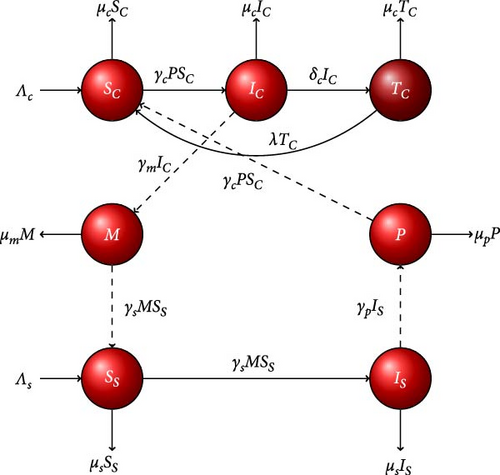
F. hepatica parasites live in three environments: free-living fasciola larvae, snails, and the cattle biological environment. The cattle population is split into three subpopulations: susceptible cattle population (S_C(t)), infected cattle population (I_C(t)), and treated cattle population (T_C(t)) at any time. The snail population is divided into two classes: susceptible and infected snails, denoted by (S_S(t)) and (I_S(t)), respectively. Similarly, fasciola larvae have two subpopulations: miracidium (M(t)) and metacercariae (P(t)).

Susceptible cattle progress to infection at a rate γ_c, by consuming metacercaria on the pasture. The infected cattle are treated at rate δ_c and the treated cattle recover at a rate λ. All susceptible, infected, and treated cattle have a natural death rate of μ_c. The infected cattle release eggs and hatch into freely floating larvae known as miracidia at rate γ_m. The portion of the miracidia population penetrates the snail at rate γ_s. Figure 1 depicts the flowchart of the fasciola hepatica transmission model.

Details are in the caption following the image — **Figure 1**
Open in figure viewer PowerPoint

Flow diagram of the fasciola hepatica disease transfer.

The model is presented using the ODE systems as follows:

()

with nonnegative initial conditions: S_C(0) ≥ 0, I_C(0) ≥ 0, T_C(0) ≥ 0, M(0) ≥ 0, P(0) ≥ 0, S_S(0) ≥ 0, and I_S(0) ≥ 0. Table 1 presents the values and biological relevance of each system parameter.

Table 1. Values and descriptions of Model (1) parameters.

Parameter	Epidemiological description	Value	Source
Λ_c	Cattle recruitment rate	67/day	[27]
Λ_s	Snail recruitment rate	3,000/day	[28]
μ_c	Cattle natural death rate	0.0185/day	[27]
μ_s	Snails natural death rate	0.001644/day	[27]
μ_m	Natural death rate for miracidia larvae	0.9/day	[28, 29]
μ_p	Natural death rate for metacercariae larvae	0.6452/day	[27]
γ_m	Rate of cattle produces miracidia	6.96/cattle/day	[28]
γ_p	Rate of snail produces metacercariae	2.6/snail/day	[28]
γ_c	Per capita infection rate of cattle	0.0000005/cyst/day	[27]
γ_s	Per capita infection rate of snails	0.00000004/miracidia/day	Assumed
δ_c	Treatment rate of infected cattle	0.65/day	Assumed
λ	Treatment efficiency of the infected cattle	0.9567/day	[27]

3. Model Analysis

3.1. Feasible Region and the Disease-Free Equilibrium Point

To ascertain that Model (1) is epidemically and mathematically well-posed, we show that all solutions with positive initial conditions remain positive at any time t > 0. Consider the total cattle population, N_C(t) = S_C(t) + I_C(t) + T_C(t), and the total snail population, N_S(t) = S_S(t) + I_S(t). From Model (1), we have

, and

. Therefore, every possible solution of Model (1) remains within the positive invariant region Ω, which is defined as follows:

()

Setting the derivatives of Model (1) to zero gives the disease-free equilibrium point as follows:

()

3.2. Local Stability of the Disease-Free Equilibrium

To analyze the stability of the disease-free equilibrium, we calculate the basic reproduction number. In epidemiological studies, the next-generation matrix technique [30] is used to quantify the basic reproduction for an infectious disease compartmental framework. The matrices

and

represent the transfer and new infection terms, respectively, which are given by the following equation:

()

After some algebraic simplification, we get the following equation

()

Therefore, the reproductive number, which is the spectral radius of

, is as follows:

()

The basic reproduction number is the anticipated number of subsequent cases resulting from a single infestation in an entirely susceptible individual. It is used to determine whether the infection extinctions or spreads throughout the population [31].

Since Model (1) satisfies axioms (A1)–(A5) of Theorem 2 in van den Driessche and Watmough [30], we have the following result.

Lemma 1. The disease-free equilibrium point is locally asymptotically stable in Ω whenever R₀ < 1 and unstable if R₀ > 1.

3.3. Global Stability of Disease-Free Equilibrium

Castillo-Chavez et al. [32] proposed a method to determine the global steady state of the DFE within

. Model (1) is expressed as follows:

()

with U = (S_C, S_S) consists of the disease-free subgroups, and V = (I_C, T_C, M, I_S, P) consists of infectious subgroups.

If the requirements (C1) and (C2) stated below are satisfied, then E₀ will be globally stable whenever R₀ < 1.

C1 When , U^∗ is globally stable.
C2 for (U, V) ∈ Ω.

B = D_VQ(U^∗, 0) is Metzler-matrix (off-diagonal entries of B are non-negative), and Ω is the set at which the system becomes feasible (see the description of the method in Kadaleka et al.’s [33] study).

Theorem 1. The disease-free equilibrium, E₀, is globally asymptotically stable if R₀ < 1 and unstable otherwise.

Proof. From Models (1) and (7), we have the following equations:

()

with

()

Clearly, is the global asymptote of Equation (8) and hence the condition C1 is satisfied. Also, from Equation (12), for and . Thus, , ∀(U, V) ∈ Ω, and condition C2 holds. Since the nondiagonal entries are nonnegative, B is an M-matrix. This demonstrates that the DFE is globally stable whenever R₀ < 1.

3.4. Existence of Endemic Equilibrium Point

Lemma 2. Model (1) has a unique endemic equilibrium for R₀ > 1.

The endemic equilibrium point

occurs when the F. hepatica infection persists in cattle. It is given by the following equation:

()

where

()

such that,

Thus, , , , M^∗ > 0, , , and P^∗ > 0 if R₀ > 1. This proves that the disease becomes endemic if R₀ > 1.

3.5. Local Stability of Endemic Equilibrium Point

Lemma 3. The endemic equilibrium point, , is locally asymptotically stable if R₀ > 1; otherwise, it is unstable.

Applying Castillo-Chavez and Song’s [34] theorem, the model exhibits a forward bifurcation (refer to the proof of Theorem 2), which ensures the endemic equilibrium is locally asymptotically stable if R₀ > 1.

3.6. Bifurcation Analysis

Bifurcation theory examines the qualitative changes in system behavior, particularly the stability or instability of fixed points and periodic orbits, as parameters vary. It is a useful tool for analyzing qualitative changes in steady-state solutions [35]. The occurrence of a forward bifurcation indicates that endemic equilibrium is locally stable if R₀ > 1 [36].

Theorem 2. Model (1) has a forward bifurcation when R₀ = 1.

Proof. We use the center manifold theorem in Appendix A to prove this theorem. For the sake of simplicity, the following change of variable is made for Model (1):

S_C = y₁, I_C = y₂, T_C = y₃, M = y₄, S_S = y₅, I_S = y₆, and P = y₇. Thus, Model (1) transforms into the following equation:

()

The disease-free equilibrium of Equation (15) is

. Assume

be the bifurcation parameter at R₀ = 1 and we obtained the following equation:

()

When

, the Jacobian matrix of Equation (15) at disease-free equilibrium gives the following equation:

()

The eigenvalues of J_ϕ are λ₁ = 0, λ₂ = −μ_c, λ₃ = −μ_s, λ₄ = −λ − μ_c, and other eigenvalues are given by the following equation:

()

where a₂ = δ_c + μ_c + μ_m + μ_p + μ_s,

a₁ = δ_cμ_m + μ_cμ_m + δ_cμ_p + μ_cμ_p + μ_mμ_p + δ_cμ_s + μ_cμ_s + μ_mμ_s + μ_pμ_s, and

a₀ = δ_cμ_mμ_p + μ_cμ_mμ_p + δ_c μ_mμ_s + μ_cμ_mμ_s + δ_cμ_pμ_s + μ_cμ_pμ_s + μ_mμ_pμ_s.

Here a₂, a₁, and a₀ are positive and a₂a₁ − a₀ > 0. Thus, the Jacobian J_ϕ(E₀) has a simple zero eigenvalue, with all remaining eigenvalues having negative real components by the Routh–Hurwitz criterion. Therefore, the center manifold theory can be used to examine the behavior of the model. Let l = (l₁, l₂, l₃, l₄, l₅, l₆, l₇) and h = (h₁, h₂, h₃, h₄, h₅, h₆, h₇) are left and right eigenvectors of J(E₀).

The left eigenvectors are obtained by multiplying l by J(E₀) and equating with 0. So after evaluating, the left eigenvector is as follows:

()

Similarly, the right eigenvector is obtained by multiplying J(E₀) by h and equating with 0. After computation, the right eigenvector is as follows:

()

The functions r₁ = Λ_c − γ_cy₁y₇ − μ_cy₁ + λy₃, r₂ = γ_cy₁y₇ − (δ_c + μ_c)y₂, r₅ = Λ_s − γ_sy₄y₅ − μ_sy₅, and r₆ = γ_sy₄y₅ − μ_sy₆ have the following nonzero partial derivatives at DFE, E₀:

()

After some calculations, the bifurcation coefficients (see the computational procedures in [37] and Appendix A) are given by the following equation:

()

Therefore, a < 0 and b > 0 for h₇ > 0 and l₂ > 0, the system exhibits a forward bifurcation at R₀ = 1 (Figure 2). A forward bifurcation at R₀ = 1 suggests that F. hepatica disease can become endemic in cattle, switching from disease-free to persistent infection.

3.7. Global Stability of Endemic Equilibrium

Theorem 3. If R₀ > 1, then the endemic equilibrium point, , is globally asymptotically stable.

Proof. The following Lyapunov function can be designed:

()

At the endemic equilibrium point, , while it is positive for all other points in the set Ω, except for this specific equilibrium point. When differentiating the function V with respect to t, we obtain the following equation:

()

Substituting the derivative of each state variable from Equation (1) into Equation (23) yields the following equation:

()

Replacing the requirement for the existence of an endemic equilibrium point provides the following equation:

()

Rearranging Equation (24) yields the following equation:

()

where

()

If A ≤ B, then , satisfying the third condition of the Lyapunov criteria. As a result, the singleton , which represents the endemic equilibrium point, becomes the largest invariant set in Ω. Therefore, based on Lasalle’s invariance principle [38], it can be concluded that is globally asymptotically stable within Ω if A ≤ B. This condition holds if and only if R₀ > 1.

4. Sensitivity Analysis

Sensitivity analysis is used extensively in epidemiology to identify the most influential parameters in the model [36]. The normalized sensitivity index that measures the percentage change of R₀ with relation to the parameter ω, denoted by

and defined as follows [39]:

()

Table 2 summarizes the sensitivity index results using the parameter values from Table 1. Figure 3 illustrates a graphical simulation of sensitivity indices. The sensitivity analysis result shows that recruitment rates, rates of producing miracidia and metacercariae, and transmission rates of cattle and snails are the most sensitive parameters with a direct influence on R₀. Biologically, the transmission rates for the snail and cattle populations, as well as the rates at which cattle produce miracidia and snails produce metacercariae, have contributed to the fasciola hepatica severity in the cattle. The positive index indicates that if the per capita infection rate of cattle (γ_c) is adjusted by 50%, the value of R₀ will similarly increase or decrease by approximately 25%.

Table 2. Normalized forward sensitivity indices.

Parameters		Sensitivity indices
Λ_c		+0.5
Λ_s		+0.5
μ_c	−(δ_c + 2μ_c)/2(δ_c + μ_c))	−0.5023
μ_s	−1	−1
μ_m		−0.5
μ_p		−0.5
γ_m		+0.5
γ_p		+0.5
γ_c		+0.5
γ_s		+0.5
δ_c	−δ_c/2(δ_c + μ_c)	−0.497698

The results also show that the mortality rates of miracidia, metacercaria, and snail populations, as well as the treatment rate of infected cattle, indirectly impact the basic reproduction number. The snail mortality rate is the most significant parameter that has an indirect effect on R₀. A 50% increase or decrease in the snail mortality rate (μ_s) will lead to an approximate 50% decrease or increase in the value of R₀, respectively. Therefore, to prevent the spread of fasciola hepatica infection in cattle, stakeholders should increase treatment rates and the mortality rates of snail, miracidia, and metacercaria populations.

5. Numerical Simulations

This section conducts simulations using the parameter values listed in Table 1 to investigate the qualitative dynamics of fasciola hepatica disease spread. While many of these parameter values are sourced from existing studies, some are proposed specifically for the simulation. Numerical simulation has been performed using MATLAB ode45 code.

5.1. The Stability Behavior of Endemic Equilibrium

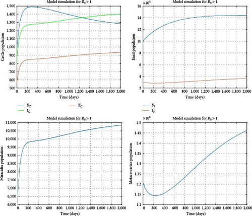
Simulations are performed for the first 2,000 days, with initial conditions set as . Using Table 1 parameter values in Model (1), we found the reproduction number, R₀ = 1.93597 > 1. Indeed, using these parameter values in Model (1), we obtain a unique endemic equilibrium point . As shown in the graphical illustrations in Figure 4, all solution trajectories of the system eventually converge to the endemic equilibrium point, . As proved by the analytic solution, the endemic equilibrium is locally stable whenever R₀ > 1. Biologically, the fasciola hepatica disease will continue to spread among susceptible hosts unless an external intervention mechanism is designed.

5.2. The Stability Behavior of Disease-Free Equilibrium

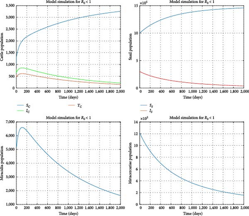
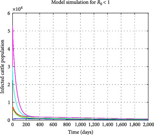
Assuming the transmission rates γ_c and γ_s are reduced to 0.0000003 and 0.00000002, respectively, the treatment rate δ_c is increased to 0.7, and the mortality rate of the snail population is elevated to 0.002. We find the reproduction number to be R₀ = 0.840751 and the disease-free equilibrium to be . Figure 5 illustrates that all model solution trajectories converge to the disease-free equilibrium (DFE) over time, indicating its local stability. Additionally, Figure 6 indicates that the number of infected cattle declines to zero over time across various initial conditions, suggesting that the DFE is globally stable. This further demonstrates that the disease will eventually be eradicated in the cattle population. In contrast, the susceptible cattle and snail populations will reach their maximum values of and , respectively. From a biological perspective, it can be concluded that fasciola hepatica disease in cattle can be eradicated when R₀ < 1. Stakeholders should aim to minimize the reproduction number as much as possible through interventions to expedite the eradication of the disease.

5.3. Contour and Surface Plots of R₀ for Combination of Parameters

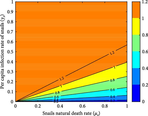
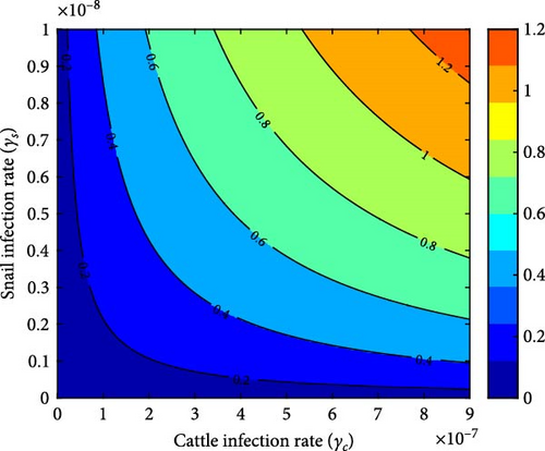
Figures 7(a), 7(b), 7(c), and 7(d) depict how the reproduction number is impacted by two control parameters, as demonstrated through the contour plots. Figure 7(a) clearly illustrates the necessity of giving utmost priority to the region below the yellow color when implementing snail control measures and proficiently managing the per capita infection rate of snails to accomplish successful eradication of the disease. When the snail death rate is low, there is an inverse relationship, causing the reproduction number to increase and the disease to persist. Figure 7(b) emphasizes the crucial role of snail and cattle infection rates in the transmission and impact of F. hepatica disease in cattle. It highlights that higher snail infection rates lead to a larger reservoir of parasites in the environment, which subsequently increases the risk of cattle exposure to the parasite. To effectively control and potentially eradicate the disease, policymakers should aim to minimize these infection rates to a level where the reproduction number is less than 1.

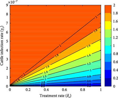
The contour plot and surface plot shown in Figures 7(c) and 8 suggest that reducing the treatment rate and cattle infection rate results in an R₀ value below one, indicating a promising approach for controlling the disease. This finding suggests that interventions targeting the treatment rate and cattle infection rate can effectively limit the spread of the disease and potentially lead to its eradication.

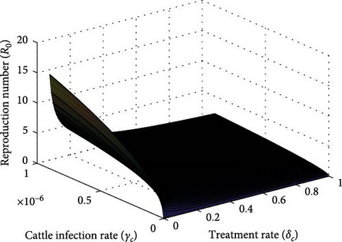
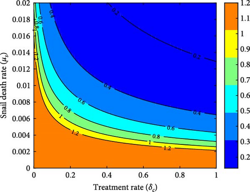
Policymakers and healthcare professionals might concentrate on establishing strategies that aim to reduce the treatment and cattle infection rates. These measures might include improving access to treatment options, implementing effective preventive measures for cattle, and adopting biosecurity protocols to minimize the risk of disease transmission. Finally, Figure 7(d) demonstrates that simultaneously improving the combined treatment rate for infected cattle and snail mortality rate leads to a lower reproduction number. Without adequate adjustments to these rates, the reproduction number remains high, indicating the persistence of the disease.

5.4. Parameter Impact on the Disease Dynamics

5.4.1. Effect of per Capita Infection Rates

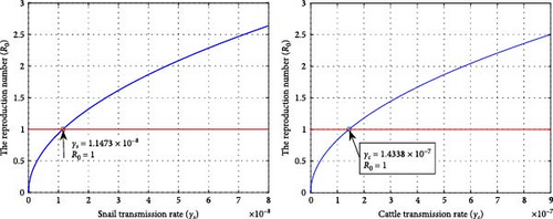
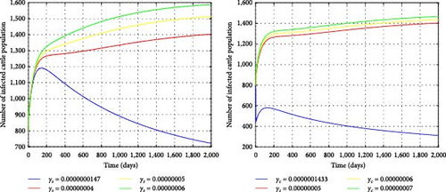
Figure 9 illustrates a graphical representation of the reproductive number in terms of disease transmission rates of cattle and snails based on parametric values in Table 1. It displays that, as the values of γ_c and γ_s increase, R₀ also increases and becomes greater than one to the right of and . This shows that disease transmission between cattle and snails significantly contributes to the endemicity of fasciola hepatica. If we consider the transmission rates lower than and , the disease will die out unless it persists. Figure 10 depicts the effects of snail transmission rate on the infected cattle using various values of γ_s = 0.0000000147, 0.00000004, 0.00000005, 0.00000006. In the same manner, by considering different values of γ_c = 0.0000001433, 0.0000005, 0.0000006, 0.0000007, the impact of per capita infection rates on cattle has been investigated. Higher infection rates in both cattle and snails lead to an increase in infected cattle. Therefore, to control the spread of the disease in the cattle population, the transmission rates for cattle and snails should be reduced to below and , respectively.

5.4.2. Effect of the Cattle Treatment Rate

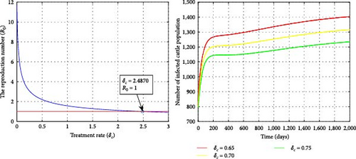
Figure 11 illustrates the impact of the treatment rate (δ_c) on R₀ and the disease epidemiology. It has been shown that as the treatment intensity increases, both R₀ and the number of infected cattle decrease. From an epidemiological perspective, improving treatment can reduce the number of infected cattle. For small values of the treatment rate, R₀ remains greater than 1. As a result, the solution graphs of the system will converge to the endemic equilibrium point, allowing the infection to persist. Increasing the treatment rate and reducing disease transmission can help decrease the incidence of fasciola hepatica infection.

5.4.3. Effect of Snail Mortality Rate

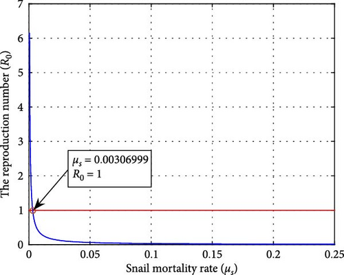
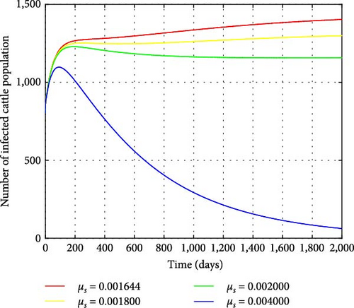
Figures 12 and 13 illustrate the impacts of the snail mortality rates (μ_s) on the reproduction number and the infected cattle population, respectively. Figure 13 shows that the number of infected cattle correspondingly decreases as the snail mortality rate increases (with values of μ_s = 0.001644, 0.0018, 0.002, 0.004). When the snail mortality rate is below μ_s = 0.00306999, the reproduction number exceeds one, allowing the F. hepatica disease to persist. Conversely, when the snail mortality rate is above μ_s = 0.00306999, R₀ falls below one, eradicating the disease. Controlling the snail population reduces cattle infection and the density of metacercariae in the ecosystem. Therefore, additional measures should be implemented to decrease the number of snails and eliminate the spread of F. hepatica in cattle.

6. Discussion

In this study, a deterministic mathematical model describing the transmission dynamics of F. hepatica disease is formulated and analyzed. The mathematical analysis and numerical simulation results show that the fasciola hepatica-free equilibrium point is locally and globally asymptotically stable if R₀ < 1. It has also been demonstrated that the endemic equilibrium point is locally and globally stable when R₀ > 1. The model exhibits a forward bifurcation. This situation happens when the fasciola hepatica-free equilibrium starts to lose its stability and a steady endemic equilibrium makes it appear while R₀ tends to increase via one. In models exhibiting forward bifurcation, having R₀ < 1 is a necessary and sufficient condition for fasciola hepatica disease eradication [40].

The sensitivity analysis is used to assess the impact of various parameters on fasciola hepatica. The results reveal that recruitment rates, transmission rates among cattle and snail populations, and shedding rates of miracidia and metacercariae directly affect the prevalence of fasciola hepatica in the cattle population. Furthermore, the mortality rates of miracidia, metacercariae, and snail populations, as well as the treatment rate of infected cattle, indirectly influence the spread of the F. hepatica parasite.

The numerical simulation results indicate that the current treatment is inadequate to prevent disease transmission within the cattle population, necessitating additional measures for disease control. Simulations also demonstrate that a strategy combining effective treatment, lower transmission rates, and higher snail mortality rates could greatly enhance disease management. This finding is consistent with a study by Diaby et al. [5], which found that the percentage of animals receiving medical treatment is not as important as combining quarantine with treatment for disease prevention. Additionally, a study by Kadaleka et al. [41] suggests that combinations of mollusciciding and therapy in a contaminated environment can effectively decrease the spread of disease, outperforming individual control methods. This integrated approach targeting both snail hosts and infected individuals could significantly reduce disease burden and improve public health outcomes, suggesting the importance of implementing such strategies in endemic regions for sustainable disease control and elimination. Therefore, stakeholders should reduce transmission rates, improve treatment rates, and increase snail population mortality rates to control this disease.

Ethical Approval

The authors agree to comply with all publication ethical standards.

Conflicts of Interest

The authors declare that they have no conflicts of interest.

Acknowledgments

Dagnaw Tantie Yihunie acknowledges the assistance provided by Debre Tabor University in conducting the research.

Appendix

A. Center Manifold Theory [34]

Assume the system is defined as follows:

()

where G(0, π) ≡ 0, for every parameter π, i.e., zero is the equilibrium of the system. Consider the following conditions:

C1 Matrix M = D_vG(0, 0) = (∂G_i/∂v_j)(0, 0) is the linearization of Equation (A.1) around the equilibrium. The simple eigenvalue of A is zero, and the other eigenvalues have real negative parts.
C2 Let M has a left eigenvector l and a right eigenvector h that corresponding to the zero eigenvalue. Suppose G_k be the kth component of G, and we have the following relation:
()

The signs of p and q, therefore, totally dictate the local behavior of System (A.1) in the neighborhood of zero:

(i)
For both positive p and q. Zero is locally stable and there is a positive unstable equilibrium if π < 0 with |π| < 1; zero is unstable and there is a negative and locally stable equilibrium, if 0 < π < 1.
(ii)
For both negative p and q. Zero is unstable, if π < 0 with |π| < 1; zero is locally stable, and a positive unstable equilibrium appears, if 0 < π < 1.
(iii)
For positive p and negative q. Zero is unstable, and there is a locally stable negative equilibrium if π < 0 with |π| < 1; zero is stable, and a positive unstable equilibrium appears, when 0 < ϕ < 1.
(iv)
For negative p and positive q. The stability of zero shifts from stable to instability, if π switches from negative to positive. A negative unstable equilibrium transforms into a positive and locally stable equilibrium.

Open Research

Data Availability

The research in this article used cited data sources and was not dependent on specific data or materials.

References

1 Logue C. M., Barbieri N. L., and Nielsen D. W., Pathogens of food animals: sources, characteristics, human risk, and methods of detection, Advances in Food and Nutrition Research. (2017) 82, 277–365, https://doi.org/10.1016/bs.afnr.2016.12.009, 2-s2.0-85011556277.
10.1016/bs.afnr.2016.12.009
CAS PubMed Google Scholar
2 Mas-Coma S., Agramunt V. H., and Valero M. A., Neurological and ocular fascioliasis in humans, Advances in Parasitology. (2014) 84, 27–149, https://doi.org/10.1016/B978-0-12-800099-1.00002-8, 2-s2.0-84892989945.
10.1016/B978-0-12-800099-1.00002-8
PubMed Web of Science® Google Scholar
3 Lalor R., Cwiklinski K., Calvani N. E. D., Dorey A., Hamon S., Corrales J. L., Dalton J. P., and De Marco Verissimo C., Pathogenicity and virulence of the liver flukes Fasciola hepatica and Fasciola Gigantica that cause the zoonosis Fasciolosis, Virulence. (2021) 12, no. 1, 2839–2867, https://doi.org/10.1080/21505594.2021.1996520.
10.1080/21505594.2021.1996520
CAS PubMed Web of Science® Google Scholar
4 Bargues M. D., Valero M. A., Trueba G. A., Fornasini M., Villavicencio A. F., Guamán R. D.;o, De Elías-Escribano A., Pérez-Crespo I., Artigas P., and Mas-Coma S., DNA multi-marker genotyping and CIAS morphometric phenotyping of Fasciola gigantica-sized flukes from ecuador, with an analysis of the Radix absence in the new world and the evolutionary lymnaeid snail vector filter, Animals. (2021) 11, no. 9, https://doi.org/10.3390/ani11092495, 2495.
10.3390/ani11092495
PubMed Google Scholar
5 Diaby M., Diop O., Nassouri E., Sène A., and Sène M., Mathematical analysis of fasciola epidemic model with treatment and quarantine, International Workshop on Complex Systems Modelling & Simulation, 2019, Springer, 133–149.
Google Scholar
6 Zewde A., Bayu Y., and Wondimu A., Prevalence of bovine fasciolosis and its economic loss due to liver condemnation at Wolaita Sodo Municipal Abattoir, Ethiopia, Veterinary Medicine International. (2019) 2019, 7, https://doi.org/10.1155/2019/9572373, 9572373.
10.1155/2019/9572373
PubMed Google Scholar
7 Ashrafi K., Valero M. A., Peixoto R. V., Artigas P., Panova M., and Mas-Coma S., Distribution of Fasciola hepatica and F. gigantica in the endemic area of Guilan, Iran: relationships between zonal overlap and phenotypic traits, Infection, Genetics and Evolution. (2015) 31, 95–109, https://doi.org/10.1016/j.meegid.2015.01.009, 2-s2.0-84922385872.
10.1016/j.meegid.2015.01.009
PubMed Web of Science® Google Scholar
8 Atalabi T. E. and Lawal O. T., Fascioliasis: a foodborne disease of veterinary and zoonotic importance, Rural Health, 2020, IntechOpen, https://doi.org/10.5772/intechopen.91361.
Google Scholar
9 Pan M., Bai S.-Y., Ji T.-K., Fan Y.-M., Liu D.-D., Yang Y., Tao J.-P., and Huang S.-Y., Epidemiology of Fasciola spp. in the intermediate host in China: a potential risk for fasciolosis transmission, Acta Tropica. (2022) 230, 231–240, https://doi.org/10.1016/j.actatropica.2022.106394, 106394.
10.1016/j.actatropica.2022.106394
Google Scholar
10 Ai L., Chen M.-X., Alasaad S., Elsheikha H. M., Li J., Li H.-L., Lin R.-Q., Zou F.-C., Zhu X.-Q., and Chen J.-X., Genetic characterization, species differentiation and detection of Fasciola spp. by molecular approaches, Parasites & Vectors. (2011) 4, https://doi.org/10.1186/1756-3305-4-101, 2-s2.0-79958154317, 101.
10.1186/1756-3305-4-101
PubMed Web of Science® Google Scholar
11 Fontenla S., Langleib M., de la Torre-Escudero E., Domínguez M. F., Robinson M. W., and Tort J., Role of Fasciola hepatica small RNAs in the Interaction with the mammalian host, Frontiers in Cellular and Infection Microbiology. (2022) 11, https://doi.org/10.3389/fcimb.2021.812141, 812141.
10.3389/fcimb.2021.812141
PubMed Google Scholar
12 Alemu B., Bovine fasciolosis in Ethiopia-a review, Journal of Veterinary and Animal Research. (2019) 2, 202.
Google Scholar
13 Ardo M. B. and Aliyara Y. H., Prevalence of Fasciolosis in small ruminants slaughtered at yola modern abattoir, Adamawa State, Nigeria, Bayero Journal of Pure and Applied Sciences. (2014) 7, no. 2, 13–16, https://doi.org/10.4314/bajopas.v7i2.3.
10.4314/bajopas.v7i2.3
Google Scholar
14 Diaz-Quevedo C., Frias H., Cahuana G. M., Tapia-Limonchi R., Chenet S. M., and Tejedo J. R., High prevalence and risk factors of fascioliasis in cattle in Amazonas, Peru, Parasitology International. (2021) 85, https://doi.org/10.1016/j.parint.2021.102428, 102428.
10.1016/j.parint.2021.102428
CAS PubMed Google Scholar
15 Mas-Coma S., Epidemiology of fascioliasis in human endemic areas, Journal of Helminthology. (2005) 79, no. 3, 207–216, https://doi.org/10.1079/JOH2005296, 2-s2.0-23944511629.
10.1079/JOH2005296
CAS PubMed Web of Science® Google Scholar
16 Caravedo M. A. and Cabada M. M., Human fascioliasis: current epidemiological status and strategies for diagnosis, treatment, and control, Research and Reports in Tropical Medicine. (2020) 11, 149–158, https://doi.org/10.2147/RRTM.S237461.
10.2147/RRTM.S237461
PubMed Web of Science® Google Scholar
17 García-López X., Jaramillo-Meza L., Quiroz-Romero H., Arriaga-Díaz C., Martínez-Maya J., Diosdado-Vargas F., and Díaz-Otero F., Effect of coinfection by Fasciola hepatica and Mycobacterium bovis on bovine tuberculosis immunodiagnosis in an enzootic area Hidalgo State, Mexico, Journal of Veterinary Healthcare. (2018) 1, no. 4, 41–54, https://doi.org/10.14302/issn.2575-1212.jvhc-18-2487.
10.14302/issn.2575-1212.jvhc-18-2487
Google Scholar
18 Opio L. G., Abdelfattah E. M., Terry J., Odongo S., and Okello E., Prevalence of fascioliasis and associated economic losses in cattle slaughtered at Lira Municipality Abattoir in Northern Uganda, Animals. (2021) 11, no. 3, https://doi.org/10.3390/ani11030681, 681.
10.3390/ani11030681
PubMed Google Scholar
19 Seid U. and Melese M., Review on prevalence, distrbution and economic significance of liver fluke in Ethiopia, ARC Journal of Animal and Veterinary Sciences. (2018) 4, no. 2, 38–48, https://doi.org/10.20431/2455-2518.0402006.
10.20431/2455-2518.0402006
Google Scholar
20 Wesołowska A., Basałaj K., Norbury L. J., Sielicka A., Wędrychowicz H., and Zawistowska-Deniziak A., Vaccination against Fasciola hepatica using cathepsin L3 and B3 proteases delivered alone or in combination, Veterinary Parasitology. (2018) 250, 15–21, https://doi.org/10.1016/j.vetpar.2017.12.007, 2-s2.0-85037653647.
10.1016/j.vetpar.2017.12.007
CAS PubMed Google Scholar
21 Admassu B., Shite A., and Kinfe G., A review on bovine fasciolosis, European Journal of Biological Sciences. (2015) 7, no. 3, 139–146.
Google Scholar
22 Barro M., Guiro A., and Ouedraogo D., Optimal control of a SIR epidemic model with general incidence function and a time delays, Cubo (Temuco). (2018) 20, no. 2, 53–66, https://doi.org/10.4067/S0719-06462018000200053.
10.4067/S0719-06462018000200053
Google Scholar
23 Turner J., Howell A., McCann C., Caminade C., Bowers R. G., Williams D., and Baylis M., A model to assess the efficacy of vaccines for control of liver fluke infection, Scientific Reports. (2016) 6, https://doi.org/10.1038/srep23345, 2-s2.0-84962301677, 23345.
10.1038/srep23345
CAS PubMed Google Scholar
24 Ogunmiloro O. M., Mathematical analysis and approximate solution of a fractional order caputo fascioliasis disease model, Chaos, Solitons & Fractals. (2021) 146, https://doi.org/10.1016/j.chaos.2021.110851, 110851.
10.1016/j.chaos.2021.110851
Google Scholar
25 León Tás M., Porco T. C., Kim C. S., Kaewkes S., Kaewkes W., Sripa B., and Spear R. C., Modeling liver fluke transmission in northeast Thailand: impacts of development, hydrology, and control, Acta Tropica. (2018) 188, 101–107, https://doi.org/10.1016/j.actatropica.2018.08.008, 2-s2.0-85052755108.
10.1016/j.actatropica.2018.08.008
PubMed Google Scholar
26 Goodall E. A., McIlroy S. G., McCracken R. M., McLoughlin E. M., and Taylor S. M., A mathematical forecasting model for the annual prevalence of Fasciolosis, Agricultural Systems. (1991) 36, no. 2, 231–240, https://doi.org/10.1016/0308-521X(91)90026-7, 2-s2.0-44949281765.
10.1016/0308-521X(91)90026-7
Google Scholar
27 Diaby M., Diop O., Nassouri E., Sène A., and Sène M., Mathematical analysis of fasciola epidemic model with treatment and quarantine, Modelling, Simulation and Applications of Complex Systems, 2021, Springer Singapore, 133–149, https://doi.org/10.1007/978-981-16-2629-6_7.
10.1007/978-981-16-2629-6_7
Google Scholar
28 Kanyi E., Afolabi A. S., and Onyango N. O., Mathematical modeling and analysis of transmission dynamics and control of schistosomiasis, Journal of Applied Mathematics. (2021) 2021, 20, https://doi.org/10.1155/2021/6653796, 6653796.
10.1155/2021/6653796
Google Scholar
29 Chiyaka E. T. and Garira W., Mathematical analysis of the transmission dynamics of schistosomiasis in the human-snail hosts, Journal of Biological Systems. (2009) 17, no. 3, 397–423, https://doi.org/10.1142/S0218339009002910, 2-s2.0-69049089967.
10.1142/S0218339009002910
Google Scholar
30 van den Driessche P. and Watmough J., Reproduction numbers and sub-threshold endemic equilibria for compartmental models of disease transmission, Mathematical Biosciences. (2002) 180, no. 1-2, 29–48, https://doi.org/10.1016/S0025-5564(02)00108-6, 2-s2.0-0036845274.
10.1016/S0025-5564(02)00108-6
CAS PubMed Web of Science® Google Scholar
31 Bakare E. A., Nwagwo A., and Danso-Addo E., Optimal control analysis of an SIR epidemic model with constant recruitment, International Journal of Applied Mathematical Research. (2014) 3, no. 3, 273–285, https://doi.org/10.14419/ijamr.v3i3.2872.
10.14419/ijamr.v3i3.2872
Google Scholar
32 Castillo-Chavez C., Feng Z., and Huang W., On the computation of R₀ and its role on global stability, Mathematical Approaches for Emerging and Re-Emerging Infection Diseases: An Introduction, 2002, 125, Springer-Verlag and Berlin-Heidelberg-New York, 229–250.
10.1007/978-1-4757-3667-0_13
Google Scholar
33 Kadaleka S., Abelman S., and Tchuenche J. M., A human-bovine schistosomiasis mathematical model with treatment and mollusciciding, Acta Biotheoretica. (2021) 69, no. 4, 511–541, https://doi.org/10.1007/s10441-021-09416-0.
10.1007/s10441-021-09416-0
PubMed Google Scholar
34 Castillo-Chavez C. and Song B., Dynamical models of tuberculosis and their applications, Mathematical Biosciences and Engineering. (2004) 1, no. 2, 361–404, https://doi.org/10.3934/mbe.2004.1.361.
10.3934/mbe.2004.1.361
PubMed Web of Science® Google Scholar
35 Sharma S., Coetzee E. B., Lowenberg M. H., Neild S. A., and Krauskopf B., Numerical continuation and bifurcation analysis in aircraft design: an industrial perspective, Philosophical Transactions of the Royal Society A: Mathematical, Physical and Engineering Sciences. (2015) 373, no. 2051, https://doi.org/10.1098/rsta.2014.0406, 2-s2.0-84941236618, 20140406.
10.1098/rsta.2014.0406
PubMed Web of Science® Google Scholar
36 Madubueze C. E., Gweryina R. I., and Abokwara A., Mathematical analysis and optimal control of schistosomiasis transmission model, Biomath Communications. (2022) 9, no. 1, https://doi.org/10.11145/bmc.2022.03.071, 2203071.
10.11145/bmc.2022.03.071
Google Scholar
37 Kadaleka S., Abelman S., and Tchuenche J. M., A mathematical model of the transmission dynamics of bovine schistosomiasis with contaminated environment, Acta Biotheoretica. (2022) 70, no. 1, https://doi.org/10.1007/s10441-021-09434-y, 9.
10.1007/s10441-021-09434-y
PubMed Google Scholar
38 LaSalle J. P., The stability of dynamical systems, Regional Conference Series in Applied Mathematics, 1976, 25, Society for Industrial and Applied Mathematics, Philadelphia, PA.
Google Scholar
39 Zamir M., Zaman G., and Alshomrani A. S., Sensitivity analysis and optimal control of anthroponotic cutaneous leishmania, PLoS ONE. (2016) 11, no. 8, https://doi.org/10.1371/journal.pone.0160513, 2-s2.0-84983071305, e0160513.
10.1371/journal.pone.0160513
PubMed Web of Science® Google Scholar
40 Gumel A. B., Causes of backward bifurcations in some epidemiological models, Journal of Mathematical Analysis and Applications. (2012) 395, no. 1, 355–365, https://doi.org/10.1016/j.jmaa.2012.04.077, 2-s2.0-84862985622.
10.1016/j.jmaa.2012.04.077
Web of Science® Google Scholar
41 Kadaleka S., Abelman S., Mwamtobe P., and Tchuenche J., Optimal control analysis of a human–bovine schistosomiasis model, Journal of Biological Systems. (2021) 29, no. 1, 1–26, https://doi.org/10.1142/S0218339021500017.
10.1142/S0218339021500017
Google Scholar

All articles

Modeling and Analysis of Fasciola Hepatica Disease Transmission

Abstract

1. Introduction

2. Model Formulation

3. Model Analysis

3.1. Feasible Region and the Disease-Free Equilibrium Point

3.2. Local Stability of the Disease-Free Equilibrium

3.3. Global Stability of Disease-Free Equilibrium

3.4. Existence of Endemic Equilibrium Point

3.5. Local Stability of Endemic Equilibrium Point

3.6. Bifurcation Analysis

3.7. Global Stability of Endemic Equilibrium

4. Sensitivity Analysis

5. Numerical Simulations

5.1. The Stability Behavior of Endemic Equilibrium

5.2. The Stability Behavior of Disease-Free Equilibrium

5.3. Contour and Surface Plots of R₀ for Combination of Parameters

5.4. Parameter Impact on the Disease Dynamics

5.4.1. Effect of per Capita Infection Rates

5.4.2. Effect of the Cattle Treatment Rate

5.4.3. Effect of Snail Mortality Rate

6. Discussion

Ethical Approval

Conflicts of Interest

Acknowledgments

Appendix

A. Center Manifold Theory [34]

Open Research

Data Availability

References

Figures

References

Information

About Wiley Online Library

Help & Support

Opportunities

Connect with Wiley

Modeling and Analysis of Fasciola Hepatica Disease Transmission

Abstract

1. Introduction

2. Model Formulation

3. Model Analysis

3.1. Feasible Region and the Disease-Free Equilibrium Point

3.2. Local Stability of the Disease-Free Equilibrium

3.3. Global Stability of Disease-Free Equilibrium

3.4. Existence of Endemic Equilibrium Point

3.5. Local Stability of Endemic Equilibrium Point

3.6. Bifurcation Analysis

3.7. Global Stability of Endemic Equilibrium

4. Sensitivity Analysis

5. Numerical Simulations

5.1. The Stability Behavior of Endemic Equilibrium

5.2. The Stability Behavior of Disease-Free Equilibrium

5.3. Contour and Surface Plots of R0 for Combination of Parameters

5.4. Parameter Impact on the Disease Dynamics

5.4.1. Effect of per Capita Infection Rates

5.4.2. Effect of the Cattle Treatment Rate

5.4.3. Effect of Snail Mortality Rate

6. Discussion

Ethical Approval

Conflicts of Interest

Acknowledgments

Appendix

A. Center Manifold Theory [34]

Open Research

Data Availability

References

Figures

References

Related

Information

5.3. Contour and Surface Plots of R₀ for Combination of Parameters