Classification of Gastrointestinal Diseases Using Hybrid Recurrent Vision Transformers With Wavelet Transform
Abstract
Gastrointestinal (GI) diseases are a significant global health issue, causing millions of deaths annually. This study presents a novel method for classifying GI diseases using endoscopy videos. The proposed method involves three major phases: image processing, feature extraction, and classification. The image processing phase uses wavelet transform for segmentation and an adaptive median filter for denoising. Feature extraction is conducted using a concatenated recurrent vision transformer (RVT) with two inputs. The classification phase employs an ensemble of four classifiers: support vector machines, Bayesian network, random forest, and logistic regression. The system was trained and tested on the Hyper–Kvasir dataset, the largest publicly available GI tract image dataset, achieving an accuracy of 99.13% and an area under the curve of 0.9954. These results demonstrate a significant improvement in the accuracy and performance of GI disease classification compared to traditional methods. This study highlights the potential of combining RVTs with standard machine learning techniques and wavelet transform to enhance the automated diagnosis of GI diseases. Further validation on larger datasets and different medical environments is recommended to confirm these findings.
1. Introduction
Gastrointestinal (GI) diseases encompass a wide range of conditions affecting the digestive system, including ulcerative disorders of the upper GI tract, inflammatory bowel diseases (IBDs) like Crohn’s disease (CD) and ulcerative colitis (UC), and various infections caused by bacteria, viruses, protozoa, and parasites [1, 2]. These diseases can be triggered by factors such as poor diet, alcohol consumption, tobacco use, and certain medications [3]. Traditional diagnostic methods for GI diseases include endoscopy, colonoscopy with biopsy for UC and microscopic colitis, and ileocolonoscopic for diagnosing CD [4]. However, these methods are invasive, time-consuming, and may lack sensitivity, leading to the development of diagnostic techniques that offer improved accuracy and efficiency in detecting and identifying human GI diseases. Nowadays, technological advancements in medical image processing are rapidly automating manual medical diagnosis techniques such as ultrasound, MRI, CT, endoscopy, etc., to identify and detect diseases in different parts of the human body, such as the colorectal [5], lumbar [6], brain [7], lung [8, 9], and others. GI diseases, in particular, are one of the most predominant diseases around the world and account for approximately 8 million deaths annually worldwide [10]. Studies from 2012 indicate that 60–70 million people in the United States are affected by GI disease each year, with around 765,000 deaths recorded in 2019 due to stomach and intestinal diseases [11, 12]. Diagnosis of GI diseases typically involves physical tests, laboratory tests, and imaging, with endoscopy being the most common imaging technique. However, physical examinations are often not useful for confirming a diagnosis of GI diseases, such as Eosinophilic GI diseases. Additionally, laboratory tests using blood, urine, and stool only have a limited role in identifying GI diseases [13]. Recent advancements in digital computing, combined with the rapid growth of artificial intelligence (AI) and computer vision, have emphasized the importance of algorithms such as artificial neural networks (ANNs) and machine learning techniques for the automated diagnosis of diseases [14, 15]. In the case of GI diseases, several deep learning and machine learning techniques have been proposed to detect and classify upper and lower intestinal, gastric, and a combination of these diseases. The study [11] proposed deep learning architectures to segment and classify GI diseases such as ulcers, polyps, and bleeding by using a recurrent convolutional neural network (CNN) as a segmentation technique. Another study [16] developed a deep CNN with transfer learning for the automated detection of GI diseases from wireless capsule endoscopy images. Despite the recent research advancements in the detection and classification of GI diseases, there remains a gap in the field that requires further research. Automated medical image segmentation has received much attention due to the time-consuming and error-prone nature of manual labeling of a large number of medical images [17]. Existing methods for the automated classification, segmentation, and detection of several GI diseases have been discussed in previous studies, but the proposed method in this paper represents a novel method for the diagnosis of GI diseases.
- •
Concatenated RVTs were employed to extract useful features from the GID endoscopy images.
- •
We employed a segmentation technique based on wavelet transform, which offers several advantages, such as multiresolution analysis, precise localization, feature extraction, robustness to noise, and computational efficiency.
- •
We compared classification algorithms including SVM, RF, BN, and LR, and an ensemble of SVM, RF, BN, and LR. We found that the ensemble classifier outperformed the others. As a result, we decided to use the ensemble classifier.
The rest of the paper is organized as follows: Section 2 presents a literature review, and Section 3 describes the materials and methods. Experimental results and discussions are reported in Section 4 and Section 5, respectively. Finally, Section 5 points out future works and concludes this paper.
2. Literature Review
This section elaborates on a literature review of the selected papers. A literature review was conducted to identify research gaps and to determine the best possible technique for GID disease detection and classification. GI diseases involve a wide range of disorders affecting the GI tract and related organs. These diseases can vary in terms of site, etiology, and severity, ranging from simple malfunctions to more serious conditions. They can affect a large number of people and are prevalent in the population. Research in this area is crucial for better understanding the pathophysiology, clinical features, and complications of GI disorders, leading to the development of improved diagnostic methods and therapeutic strategies. IBDs are a subset of GI disorders characterized by a dysregulated immune response to the gut microbiome. They include CD, UC, and microscopic colitis. These conditions primarily affect the GI tract, causing symptoms such as diarrhea, abdominal pain, and weight loss. Diagnosis typically involves colonoscopy with biopsy, and treatment options have expanded to include biologic drugs targeting inflammation. Surgery may be necessary for complications or refractory disease. GI diseases encompass various benign and malignant pathologies of the digestive tract, liver, biliary tract, and pancreas [18]. Common GI disorders include gastroesophageal reflux disease, diarrhea, IBD, colorectal cancer, irritable bowel syndrome, and liver transplantation. These conditions can cause symptoms even when the GI system appears healthy. Treatment options vary depending on the specific disorder and may involve medications, dietary management, or surgical intervention [19]. In veterinary medicine, GI diseases such as IBD and pancreatitis are significant causes of chronic diarrhea and vomiting in dogs and cats. Treatment for IBD typically involves immunosuppressive therapy, antibiotics, and dietary management, while pancreatitis requires early caloric support and antiemetics for symptom management.
GI disease detection can be improved through the use of deep learning techniques such as CNNs and ANNs [20–22]. These methods analyze endoscopy images and extract features to accurately diagnose various GI diseases.
The paper [20] discusses the use of deep learning techniques, specifically CNNs, for the detection of GI diseases using endoscopy. It mentions that the proposed framework achieved an accuracy of 88.05% in disease detection using GI disease Endoscopy images. However, their approach is computationally intensive and requires extensive training data, making it less suitable for real-time applications. The paper [21] discusses the use of hybrid techniques, including ANNs and deep learning models, for diagnosing GI diseases based on endoscopy images. It does not provide specific details about the detection process. The paper claims that DenseNet-121 SVM achieved high accuracy for diagnosing various GI diseases while VGG-16 SVM also achieved good accuracy for diagnosing GI diseases. The paper [22] proposes a concatenated neural network model using VGGNet and InceptionNet to develop a GI disease diagnosis model. The model achieves a classification accuracy of 98% and Matthews’s correlation coefficient of 97.8%. Despite its effectiveness, this method struggles with images that have low contrast or significant artifacts, limiting its applicability across different imaging modalities. The paper [23] proposes a collaborative, noninvasive diagnostic scheme for the detection of GI diseases using key metabolite signatures that were identified with functional relevance to GI disease. The combined signatures achieved a discrimination area under the curve (AUC) of 0.88.rum metabolite signatures and magnetically controlled capsule endoscopy. However, the paper needs improvement with regard to its accuracy in detecting disease. The paper [24] proposes a multiclass classification framework called GI-Net for screening GI diseases using endoscopy images. It achieves 88% accuracy in diagnosing unseen images and is more effective compared to other deep learning networks. Even though the developed architecture claimed it is highly effective compared to other deep learning networks, but 88% accuracy on unseen data is poor compared to other existing models. This literature review highlights the increasing significance of leveraging technological advancements, particularly in the realm of medical image processing and AI, for the detection and classification of GI diseases. Despite the considerable progress made in recent years, particularly with the emergence of deep learning architectures and machine learning techniques, there remains a pressing need for further research to address existing challenges and gaps in the field. The proposed method presented in this study represents a novel approach toward the automated diagnosis of GI diseases, integrating RVTs with standard machine learning classifiers and wavelet transform-based segmentation. The contributions of this study lie in the employment of concatenated RVTs for feature extraction, the utilization of wavelet transform for segmentation, and the comprehensive comparison of classification algorithms, culminating in the selection of an ensemble classifier for enhanced performance. Moving forward, future research endeavors should aim to explore avenues for refining and optimizing the proposed methodology, as well as investigating the integration of additional data modalities and advanced computational techniques.
3. Materials and Methods
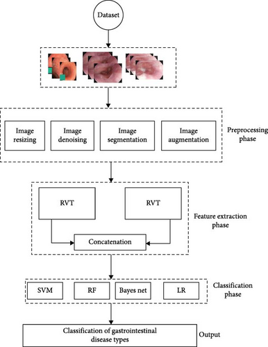
The proposed methodology for the classification of GI diseases is composed of three major phases: image processing, feature extraction, and classification. The image processing phase involves the use of wavelet transform for segmentation and adaptive median filter (AMF) for image denoising to enhance the quality of the input images. In the feature extraction phase, a concatenated RVT with two inputs is used to extract relevant features from the processed images. Finally, in the classification phase, an ensemble of four classifiers (SVM, BN, RF, and LR) is used to classify the images into different GI disease classes. The system structure is designed to effectively utilize the strengths of the two input modalities, the concatenated RVT and the ensemble of classifiers, to provide improved classification performance compared to traditional methods. The overall system architecture is illustrated in Figure 1.
3.1. Dataset
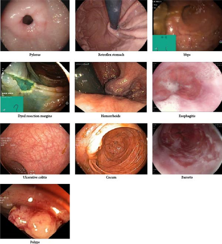
In this work, we utilized the publicly available Hyper–Kvasir dataset. The Hyper–Kvasir dataset is a comprehensive collection of endoscopy images and videos, each annotated and verified by experienced medical doctors specializing in endoscopy. It encompasses several classes depicting anatomical landmarks, pathological findings, and endoscopic procedures within the GI tract. These classes include hundreds of images each, making the dataset suitable for various tasks such as image retrieval, machine learning, deep learning, and transfer learning. The dataset features a wide range of anatomical landmarks, such as the Z-line, pylorus, and cecum, as well as pathological findings like esophagitis, polyps, and UC. Additionally, it includes images related to the removal of lesions, such as “dyed and lifted polyp” and “dyed resection margins.” The images vary in resolution from 720 × 576 to 1920 × 1072 pixels and are organized into separate folders named according to their content. Some images in the dataset include a green picture-in-picture illustrating the position and configuration of the endoscope within the bowel, provided by an electromagnetic imaging system (ScopeGuide, Olympus Europe). This additional information can support the interpretation of the images but must be carefully managed when detecting endoscopic findings. The Hyper–Kvasir dataset is extensive and well-suited for a range of computational tasks. However, it has limitations, such as potential biases in the types of GI conditions represented and possible human error in the manual assessment process. Additionally, the dataset may lack representation of rare or less commonly documented GI diseases, which could impact the model’s ability to generalize across all possible conditions. Sample images from the dataset are shown in Figure 2.
3.2. Preprocessing
Effective image preprocessing is essential for improving data quality and interpretability, thereby enhancing the accuracy and reliability of subsequent analysis. In this study, the dataset was divided into two parts: 80% for training and validation and 20% for testing. As part of the preprocessing, the images were resized to a uniform dimension to ensure consistency across the dataset. Following this, an AMF was applied for denoising, and a wavelet transform was used for segmentation. Using the Haar wavelet (equivalent to Daubechies “db1”) as the basis function, the wavelet transform was performed to a specified number of levels. These preprocessing steps were designed to reduce noise and highlight relevant features, ultimately ensuring more precise and dependable outcomes in the image analysis stages.
3.2.1. Extracting Frames
the dataset contains 11.62 h of labeled video. 12,435 JPEG images are extracted for 10 classes of GI diseases. The images are 224 by 224 RGB color scale.
3.2.2. Image Resizing
In order to optimize the efficiency of the proposed model, the extracted images are resized to a standard size of 64 × 64 RGB. This process of image resizing plays a crucial role in image processing, as it minimizes the image file size, facilitating easier storage, transfer, and manipulation.
3.2.3. Image Denoising
AMF is a nonlinear image filtering technique that has been widely used in various image processing applications. AMF has gained popularity due to its ability to effectively remove salt-and-pepper noise while preserving the edges and fine details of the image. One of the main advantages of AMF is its ability to adapt to different levels of noise in the image. Unlike traditional median filter, AMF adjusts the size of the window used for filtering based on the local noise level, making it an effective filter for images with varying levels of noise. For instance, in regions with high noise density, a larger window size is used to ensure that the median value represents the majority of the pixels in the region. In contrast, in regions with low noise density, a smaller window size is used to preserve the image details. AMF has also been shown to be effective in preserving edges and fine details in the image. Unlike linear filters such as mean and median filters, AMF does not blur the edges and fine details of the image, making it an attractive filter for applications that require edge preservation. In addition, AMF has been compared with other non-linear filters, such as the morphological filter, fuzzy filter, and the adaptive filter, and has been shown to outperform these filters in terms of noise reduction and edge preservation (Algorithm 1).
-
Algorithm 1: Adaptive median filter for denoising.
-
Procedure: ADAPTIVEMEDIANFILTER (img, window_size)
-
Input:
-
• img: Input image
-
• window_size: Size of the window for the median filter
-
Output:
-
• filtered_img: Denoised image
-
Step-by-Step Algorithm:
-
1. Initialize:
-
• filtered_img ← zero array with the same shape as img
-
• pad_size ← window_size //2
-
• padded_img ← pad img with pad_size along both horizontal and vertical axes
-
2. Iterate Over Each Pixel in the Image:
-
• For each pixel in img:
-
1. Extract Window:
-
• window ← extract the window of pixels from padded_img centered at the current pixel with size window_size
-
2. Compute Median:
-
• window_median ← compute the median value of window
-
3. Compute Absolute Differences:
-
• window_abs_diff ← compute the absolute differences between window and window_median
-
• median_abs_diff ← compute the median of window_abs_diff
-
4. Compute Threshold:
-
• Threshold ← 0.67 ∗ median_abs_diff if median_abs_diff ≠ 0, else 0.5 ∗ median of the absolute differences between the window and window_median
-
5. Update Pixel Value:
-
• If the absolute difference between the current pixel value and window_median is greater than Threshold:
-
• filtered_img[current_pixel] ← window_median
-
• Else:
-
• filtered_img[current_pixel] ← original value of the current pixel in img
-
3. Return Result:
-
• Return filtered_img
-
End procedure
3.2.4. Segmentation
This study performs wavelet transform-based image segmentation on an RGB image. Initially, the image is loaded, and then it is converted into grayscale. Thereafter, the two-dimensional wavelet transform is applied, using the Haar wavelet as the basis function. The high-frequency coefficients of the image, which represent the edges and details, are thresholded to zero to remove the noise and amplify the contrast between different regions in the image. Following this, the modified coefficients are employed to reconstruct an approximation of the initial grayscale image with the high-frequency components removed. The segmentation approach implemented in this study leverages the fact that the wavelet transform decomposes an image into different frequency bands. The high-frequency components, which correspond to edges and details, are removed by thresholding to enhance the contrast between different regions in the image. Figure 3 shows segmented images using the wavelet segmentation technique, while Algorithm 2 and Algorithm 3 demonstrate wavelet transform for segmentation and denoising, respectively.

-
Algorithm 2: Wavelet transform for segmentation.
-
Procedure: WAVELETTRANSFORM (img, level)
-
Input:
-
• img: Input image
-
• level: Number of decomposition levels for the wavelet transform
-
Output:
-
• segmented_img: Segmented image
-
Step-by-Step Algorithm:
-
1. Perform Initial Discrete Wavelet Transform:
-
• coeffs ← perform the Discrete Wavelet Transform (DWT) on the input image using the Haar wavelet (“db1”)
-
• cA, cH, cV, cD ← extract the approximation coefficients and the horizontal, vertical, and diagonal detail coefficients from the DWT coefficients
-
2. Iterate Over Levels:
-
• For i in range (level-1):
-
1. Perform DWT on Approximation Coefficients:
-
• coeffs ← perform the DWT on cA using the Haar wavelet (“db1”)
-
• cA, cH, cV cD ← extract the approximation coefficients and the horizontal, vertical, and diagonal detail coefficients from the DWT coefficients
-
3. Compute Threshold:
-
• threshold ← compute the global threshold using Otsu’s method on cA
-
4. Threshold Approximation Coefficients:
-
• segmented_img ← threshold cA to create a binary mask
-
5. Return Result:
-
• Return segmented_img
-
End procedure
-
Algorithm 3: Denoise and segment.
-
Procedure: DENOISEANDSEGMENT (img, window_size, level)
-
Input:
-
• img: Input image
-
• window_size: Window size for the adaptive median filter
-
• level: Decomposition level for the wavelet transform
-
Output:
-
• denoised_img: Denoised image
-
• segmented_img: Segmented image
-
Step-by-Step Algorithm:
-
1. Check Inputs:
-
• Ensure img is a valid image (numpy array).
-
• Ensure window_size is a positive integer.
-
• Ensure level is a positive integer.
-
2. Denoise the Image:
-
• Apply ADAPTIVEMEDIANFILTER (img, window_size) to get denoised_img.
-
3. Segment the Image:
-
• Apply WAVELETTRANSFORM (denoised_img, level) to get segmented_img.
-
4. Return Results:
-
• Return denoised_img, segmented_img.
-
End procedure
The general mathematical formula for the wavelet transform used for image segmentation is as follows:
3.2.5. Data Augmentation
The data underwent preprocessing prior to being subjected to various random transformations such as rotation, shearing, and resizing to avoid overfitting and enhance the model’s performance. The magnitude of rotation, horizontal and vertical shifts, shear angle, and zoom level were precisely controlled using predetermined parameters.
3.3. Feature Extraction
VTs are a type of neural network architecture that has been applied to various computer vision tasks such as image classification, object detection, and scene text recognition [25–27]. VTs are based on the transformer architecture, which was originally designed for natural language processing tasks [28]. VTs treat an image as a sequence of patches or features and apply the transformer architecture to these sequences [25].
In feature extraction, VTs use self-attention mechanisms to weigh the importance of different image patches and generate a representation of the image [25]. This representation can then be used as input for downstream tasks such as classification or detection [27]. The advantages of VTs include their ability to handle large inputs and capture long-range dependencies between features, their capacity for end-to-end training, and their ability to be trained on large datasets [25, 28]. Additionally, VTs can be easily adapted to different tasks and architectures, making them versatile and widely applicable [26]. RVTs are a variant of the VT architecture that adds a recurrent mechanism to the model. The recurrent mechanism enables the RVT to maintain an internal state that can capture information from previous image patches, making it well-suited for tasks that require a memory of previous image information. The advantage of RVTs over traditional VTs is their ability to capture the temporal relationships between image patches, making them well-suited for tasks such as video classification, where the order of frames is important [29]. Additionally, RVTs have been shown to outperform traditional VTs on tasks such as action recognition and scene segmentation, demonstrating their effectiveness in capturing temporal information [29, 30].
3.4. Evaluation Techniques
3.4.1. Accuracy
3.4.2. AUC
AUC is a commonly used performance metric for machine learning classification problems, which evaluates the overall performance of a classifier. In binary classification, a classifier outputs a predicted probability for each sample to belong to one of two classes, positive or negative. The AUC is the area under the receiver operating characteristic (ROC) curve, which plots the true positive rate (TPR) against the false positive rate (FPR) for different classification thresholds.
3.5. Classification
Ensemble methods are an important concept in the field of machine learning and have been widely used to improve the performance of various algorithms. These methods involve combining multiple models to make predictions and have been shown to achieve improved accuracy compared to individual models. In this article, we will discuss the recent advancements in ensemble methods and their advantages. Medical image classification is an important problem in the field of medicine, where accurate diagnosis is crucial [31]. Ensemble methods are an important concept in the field of machine learning and have been widely used to improve the performance of various algorithms. The recent advancements in ensemble methods have demonstrated their potential for achieving improved accuracy and reducing overfitting. These methods are especially useful for problems in the field of medicine, where accurate predictions are crucial [32, 33].
3.6. Hardware and Software Specifications
The hardware setup for this study featured an Intel (R) Core (TM) i5-10210U multicore CPU with a peak turbo frequency of 4.2 GHz. Our software configuration was centered around Python 3.9.13, supported by several key libraries and frameworks. We used Keras 2.11.0 for developing and training deep learning models, scikit-learn 1.0.2 for executing various machine learning tasks, and OpenCV for handling image processing and computer vision tasks. These software versions were selected to ensure compatibility, robustness, and efficiency throughout the experiments.
4. Results
4.1. Performance Evaluation of Single RVT With Standard Machine Learning Classifier
Grid Search was utilized to evaluate various hyperparameters before training each machine learning classifier. For SVM, a C value of 10, a γ of 0.001, and an RBF kernel were used. The RF classifier was trained with an entropy criterion, a maximum depth of 4, log2 maximum features, and 16 estimators. The BN was optimized with a maximum of three parent nodes per node and the Bayesian information criterion (BIC) for scoring. The performance of each machine learning algorithm was evaluated based on accuracy and AUC (area under the ROC curve), as shown in Table 1. The classification results for GI diseases using individual standard machine learning methods are presented in Table 1. These results indicate that most standard machine learning methods achieved remarkable classification performance, with AUC values ranging from 0.6787 to 0.8701 and accuracy values ranging from 68.93% to 86.06%. All standard machine learning models, except for LR, performed well. Notably, the SVM classifier outperformed other standard classifiers, achieving an accuracy of 86.06% and an AUC score of 0.8701.
| Classifier | Accuracy (%) | AUC |
|---|---|---|
| RF | 79.23 | 0.8076 |
| SVM | 86.06 | 0.8701 |
| BN | 85.1 | 0.8388 |
| LR | 68.93 | 0.6787 |
4.2. Performance Evaluation of Single RVT With Standard Ensemble Classifier
The performance of a single RVT in classifying GI data was evaluated using the AUC and accuracy metrics. The ensemble of standard ML classifiers produced an accuracy of 89.54% and an AUC of 0.9032. This result was significantly better than that of the individual weak learners. The findings are presented in Table 2.
| Classifier | Accuracy (%) | AUC |
|---|---|---|
| Ensemble | 89.54 | 0.9032 |
4.3. Performance of Concatenated RVT With Each Standard Machine Learning Classifier
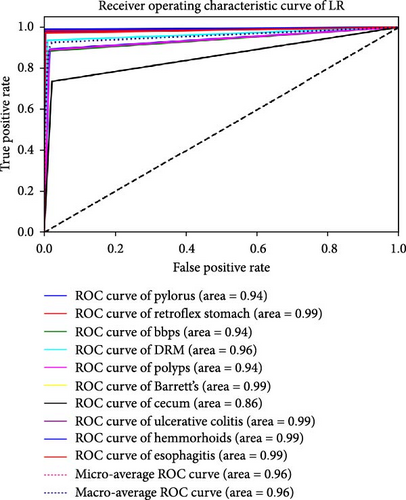
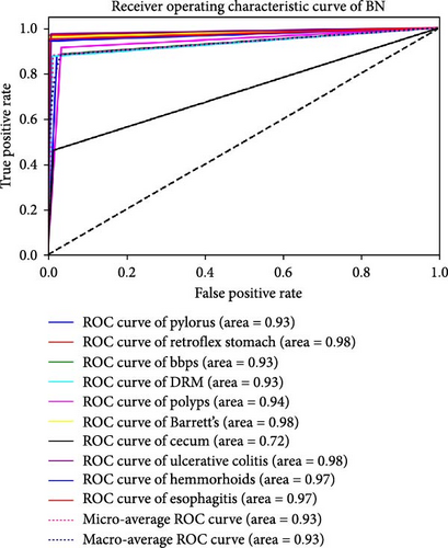
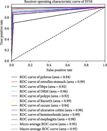
The performance of each standard machine learning model was evaluated after concatenation with the RVT. The results indicate that the accuracy and AUC of GI disease classification significantly improved after concatenating the two RVTs. The AUC and accuracy values range from 0.93 to 0.98 and from 91.88% to 98.23%, respectively. The optimal hyperparameters for each classifier were as follows: SVM with C = 100, γ = 0.0001, and an RBF kernel; RF with an entropy criterion, a maximum depth of 4, log2 maximum features, and 32 estimators; and BN with a maximum of three parent nodes per node and BIC for scoring. It was observed that when standard ML models were trained solely on endoscopy images, the best classification performance was achieved using the RF classifier, with an AUC of 0.98 and an accuracy of 98.23%. These findings are presented in Table 3. Furthermore, the results of each classifier are plotted using ROC curves in Figure 4.

| Classifier | Accuracy (%) | AUC |
|---|---|---|
| RF | 98.23 | 0.98 |
| SVM | 94.59 | 0.95 |
| BN | 91.88 | 0.93 |
| LR | 97.09 | 0.96 |
4.4. Performance of Concatenated RVT With Ensemble Classifier
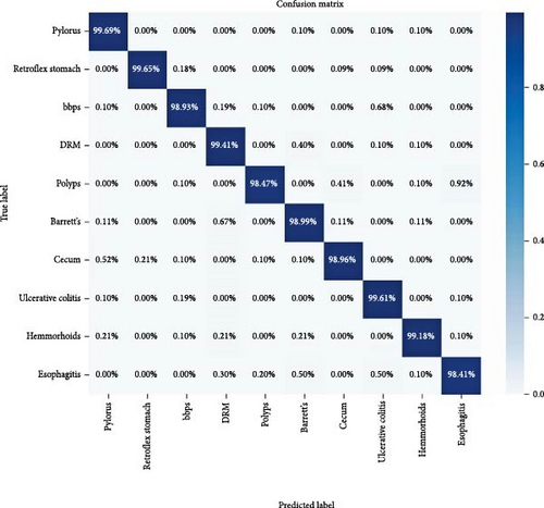
The final experiment was conducted using a concatenated RVT with an ensemble of four standard machine learning algorithms: RF, SVM, BN, and LR. For the SVM, we used a C value of 100, a γ of 0.001, and an RBF kernel. The RF classifier was trained with an entropy criterion, a maximum depth of 8, log2 maximum features, and 32 estimators. The BN was optimized with a maximum of three parent nodes per node and the BIC for scoring. The results indicate that this approach achieved an accuracy of 99.13% and an AUC score of 0.9954, as shown in Table 4. Further details on the model’s classification performance for GI disease types are presented using a confusion matrix in Figure 5. The model achieved a minimum classification accuracy of 98.41% for esophagitis and a maximum accuracy of 99.69% for pylorus.
| Classifier | Accuracy (%) | AUC |
|---|---|---|
| Ensemble | 99.13 | 0.9954 |
4.5. Comparison of Proposed Model With Other Related Works
In this section, we discuss a comparison of our proposed approach with five recently published works that have state-of-the-art results for GI disease classification, as shown in Table 5. Our proposed model, utilizing a concatenated RVT, achieved significantly superior results compared to the other related works, with an accuracy score of 99.13% and an AUC score of 0.9954. Notably, the proposed model excelled in its AUC value, indicating its superior ability to accurately identify images in the positive class while minimizing misclassification in the negative class. All the comparative works in Table 5 have used the same publicly available dataset, the Hyper–Kvasir dataset. This ensures that the comparison is fair and that the observed differences in performance are attributable to the methodologies employed rather than variations in the dataset.
| Experiments | Objective | Method | Accuracy (%) | AUC |
|---|---|---|---|---|
| Ramamurthy et al. [34] | Gastrointestinal disease classification | Efficient Net B0 with custom CNN | 97.99 | 0.9749 |
| Wong, Wong, and Chan [35] | Gastrointestinal disease classification of three types of GID | Deep transfer learning | 94 | — |
| Escobar et al. [36] | Detection of GID | VGG16 with transfer learning | 98 | — |
| Sivari et al. [37] | Gastrointestinal tract findings detection and classification | Bi-level stacking ensemble approach | 98.53 | — |
| Nouman Noor et al. [38] | Gastrointestinal disease classification | Deep learning with transfer learning | 96.40 | — |
| Proposed | Classification of GID | Concatenated RVT with ensemble | 99.13 | 0.9954 |
5. Discussion
The results of the performance evaluation of the proposed model for GI disease classification showed significant improvement compared to standard machine learning classifiers and related works. The single RVT with the standard machine learning classifiers showed good results, but the performance was significantly improved when the RVT was concatenated with the standard machine learning classifiers. The ensemble classifier with the concatenated RVT produced the best results, with an accuracy of 99.13% and an AUC of 0.9954. These results indicate that the RVT effectively extracted important features from the endoscopy images, which improved the performance of the standard machine learning classifiers. Moreover, the results showed that the concatenation of the two RVTs improved the performance even further. The comparison with related works showed that the proposed model outperformed other models in terms of accuracy and AUC. This highlights the effectiveness of the proposed approach in classifying GI diseases from endoscopy images. However, there are some limitations to this study that must be considered. First, the model was trained and tested on the Hyper–Kvasir dataset, which, while comprehensive, may not encompass all variations and complexities of GI diseases encountered in different populations and medical environments. This may limit the generalizability of the findings. Second, the computational resources required for training the RVT and the ensemble of classifiers are substantial. This could pose challenges for implementation in resource-constrained settings. Additionally, the model’s reliance on endoscopy videos means that its application is limited to environments where such imaging technology is available, potentially excluding regions with limited medical infrastructure. For future research, several directions are worth exploring. First, validating the proposed model on larger and more diverse datasets from different medical environments would help confirm its generalizability and robustness. Integrating additional data modalities, such as patient demographics, clinical history, and genetic information, could enhance the model’s diagnostic accuracy. Moreover, optimizing the computational efficiency of the model to make it more accessible in resource-limited settings would be beneficial. Investigating the interpretability of the model’s predictions could also provide valuable insights for clinical decision-making. Lastly, exploring the integration of this model with other diagnostic tools and its impact on clinical workflows could pave the way for its practical application in healthcare settings. Overall, the proposed model with the concatenated RVT and the ensemble classifier produced state-of-the-art results for GI disease classification and showed great potential for future applications in medical imaging. Nonetheless, addressing the identified limitations and exploring the suggested research directions will be crucial for realizing the full potential of this approach in improving the automated diagnosis of GI diseases.
6. Conclusion
In conclusion, this study presents a novel method for the classification of GI diseases using endoscopy videos. The proposed methodology combines RVTs and standard machine learning techniques with wavelet transform. The results of the experiments demonstrate the effectiveness of the proposed method in improving the accuracy and AUC of GI disease classification. The highest accuracy and AUC scores of 99.13% and 0.9954, respectively, were achieved when the RVT was concatenated with an ensemble of four standard machine learning algorithms. These results suggest that the proposed method has the potential to be a valuable tool in the automated diagnosis of GI diseases. However, further studies are required to validate the results on larger datasets and in different medical environments.
Ethics Statement
This retrospective study uses previously collected data for analysis in accordance with ethical standards and privacy regulations.
Consent
The authors declare that they are in agreement with this submission and for the paper to be published if accepted.
Conflicts of Interest
The authors declare no conflicts of interest.
Funding
The authors have no funding to report.
Open Research
Data Availability Statement
The data are available at the following link: https://datasets.simula.no/hyper-kvasir/.


