1. Introduction

Irradiance (G) and temperature (T) data availability have been major challenges in Bambili, Cameroon. This scarcity of data has decreased the rate of implementation of PV systems and increased the use of nonrenewable sources of energy. Photovoltaic systems still confront several obstacles because of atmospheric variations and the unpredictability of PV systems [1]. The most crucial parameters to consider when evaluating the output and efficiency of a PV system are irradiance, expressed as the power density of solar radiation that reaches the photovoltaic device, and cell temperature [2]. It is advantageous to take temperature and irradiance into account as PV performance metrics because of the strong relationship that exists between PV power and atmospheric factors. Therefore, in order to optimize the entire operation and boost the economic feasibility of PV systems, there is a need to create trustworthy mathematical models to determine their performance parameters (irradiance and temperature) [3].

In practical terms, pyranometers are tools often employed for measuring irradiance [4]. Pyranometers’ main drawbacks are their expensive nature, consisting of many sensors, and the requirement for the equipment to face towards the PV modules [5]. The use of pyranometers to assess irradiance is still uncommon in large areas like Bambili, Cameroon. On the other hand, meteorological stations for recording these data are also not available in Bambili. To an extent, the irradiance data for Bambili, Cameroon, are mostly obtained from other meteorological websites, such as NASA. However, these NASA data are mostly nonreal ground data since they are atmospheric data obtained from faraway satellites [6]. Such data might be of less use in sizing real-time PV systems. To increase PV system performance, precise methods for estimating solar irradiance must be developed [7]. Therefore, there is a need to use mathematical models to estimate the irradiance and temperatures of a particular location, which will approximate the real ground data.

Estimating irradiance and temperature is fundamental to several fields, including climatology, quality control, building automation, meteorology, and most importantly, PV applications. Temperature and irradiance readings are very important for researchers, independent test facilities, or factory producers to verify the advertised specifications of the equipment [3, 5]. In order to predict the alternating current (AC) output of PV systems and connect the electrical characteristics of the system to its operating points, it is necessary to have knowledge of the module temperature and solar radiation levels [8]. Furthermore, power-generating plants can increase the incorporation of PV energy output into the grid via the electrical network by optimizing energy management based on the knowledge of future yields from PV installations. This yield depends mostly on the amount of irradiance and temperature levels of the PV module [9].

2. Literature Review

This discussion included various mathematical and day-of-the-year-based models to determine irradiance on level and tilt surfaces, temperature at various sites, as well as energy output. A technique for calculating irradiance on flat and tilted south-oriented surfaces was presented in [10]. Utilizing certain meteorological data from Port Harcourt, Nigeria, the Duffie and Beckman model was used to estimate irradiance on tilted and horizontal surfaces. The deduced irradiance statistics for the city demonstrate that the potential of irradiance is higher during the dry season than in the wet season. An irradiance model based on an artificial neural network was formulated in [11]. They employed the daily mean of irradiance to forecast hourly data, with 43,800 hourly irradiance data points used in the training and validation of the model in Matrix Laboratory (MATLAB). This model showed better performance compared to other models based on statistical methods. In the conference proceedings held in the city of Framantum, North Cyprus, emphasis was laid on irradiances as the primary parameter that gives knowledge about the region’s PV energy potential [12]. As a result, this parameter is critical for effective PV system optimization. However, a straightforward estimating method for irradiance on tilt and level surfaces was created in order to enable the assessment of the quantity of thermal energy at every instant getting inside a complex environment supplied with PV output [13]. The acquired irradiance values demonstrated adequate agreement with the NASA database’s reference data. A strong sunshine hour irradiance model was developed in Egypt to determine the average irradiance using computed irradiance data available in the different parts of the country. The model developed employed simple formulae for irradiance, considering the variations in time and sites. They suggested that technicians and practitioners involved in PV systems could employ the model for predicting irradiance [11, 14]. Furthermore, across three locations on Malaysia’s east coast, mathematical irradiance models obtained from reviews were employed to determine the monthly averages [15]. The models proposed by Collares-Pereira and Rabl performed better for all three of the sites, according to their findings [16]. Nevertheless, the estimations of irradiance using the original linear Angstrom–Prescott (A-P) model were shown in [17]. Their findings demonstrated that the goodness of fit among the first-, second-, and third-order models was quite close. They indicated that the model coefficients related strongly with the site elevation; hence, the estimated formulae for coefficients depend entirely on these relationships [17]. The use of daily peak and lowest temperatures for evaluating the performance of four models in determining the hourly environmental temperatures in various agroecological zones throughout the year was shown in [18]. Their findings also showed that in most of the locations, the SOYGRO and Temperature models predicted hourly environmental temperature better compared to other temperature models. Because of climate change, buildings that are planned today must be used in future climatic circumstances. In comparison to previous algorithms that only used the daily peak and trough temperatures, they developed an efficient program for deducing values of hourly temperature with the help of climatic parameters in the United Kingdom [19]. A combined solar-diesel-battery energy system was modeled in [20], with the purpose of electrifying typical rural families and schools in isolated regions of Cameroon’s far north region. Using PV model equations, they estimated the energy received by titled and south-oriented modules from the horizontal irradiance of Garoua. It was demonstrated that solar panels with ratings between 50 and 180 Wp generated energy between 78.5 and 315.2 kWh annually.

3. Data and Methods

3.1. Study Site

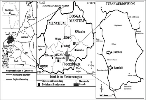
Bambili is situated in the Tubah subdivision in the Mezam division of Cameroon’s northwest region. Geographically, it is located at latitude 5.98 and longitude 10.26, with an altitude of 1474 m above sea level. Figure 1 shows the geographical map.

3.2. Estimation of Irradiance Using Different Models for Bambili

3.2.1. Model 1: A-P Model

Kaplanis and Collares-Pereira and Rabl models require average daily irradiance (H) values for any selected location. The historical H values for Bambili were not available to completely determine the values of the parameters of these models. Hence, H values were computed for any day, n of the year using the A-P model linear regression equation as follows:

$$ ()

where H is the mean daily irradiance (Wh/m²/day²), H₀ is the mean daily extraterrestrial irradiance (Wh/m²/day), S is the mean estimated daylight length (hours) for the day, S₀ is the mean peak length of daylight in hours (h) for the day, and p and q are relational parameters (Angstrom coefficients), which are geographically dependent.

• 1.

  Determination of A-P coefficients:

The empirical parameters p and q of the A-P model are usually determined by calibrations. These calibration methods, in most cases, required historical data on the concept concerning the study site, and Bambili lacked such data. However, these coefficients relate strongly with the elevation of the site and were computed as follows:

$$ ()

$$ ()

Consequently, q was obtained as

$$ ()

With an elevation of 1474 m, we obtained p = 0.1811 and q = 0.5657 for Bambili.

• 2.

  Determination of the mean daily extraterrestrial irradiance (H):

The extraterrestrial irradiance (G₀) was computed as

$$ ()

where G₀ represents the extraterrestrial irradiance,  G_C = 1367 W/m² represents the irradiance factor, and n is the day number of the year beginning from January 1 to December 31.

The declination angle (δ) is as follows:

$$ ()

The hour angle (ω_s) is as follows:

$$ ()

where ω_s represents the hour angle for the day and φ is the latitude of the study site.

• 3.

  The mean peak length of daylight in hours (h):

$$ ()

with the average sunshine hour per day for Bambili being S = 6.7.

The mean daily extraterrestrial irradiance (H₀) was obtained as follows:

$$ ()

With the obtained average daily values of irradiance from the A-P model, we further estimated the hourly irradiance.

3.2.2. Model 2: Kaplanis Model

The mathematical formulation of this model was described in [22]. This model has two parameters, a and b, which require boundary conditions and average daily irradiance values for their determination. Given that G(t) is the irradiance in watts per square meter, then it can be obtained as follows:

$$ ()

where  t is the hour of the day starting from sunrise (t_sr) to sunset (t_ss).

At the boundary condition,  t = t_ss, G(t_ss) = 0, then one established from Equation (10) that

$$ ()

To establish the second relationship between the two parameters, Equation (10) was integrated over time, with  t_sr ≤ t ≤ t_ss to obtained values of the mean daily irradiance (H) as

$$ ()

$$ ()

$$ ()

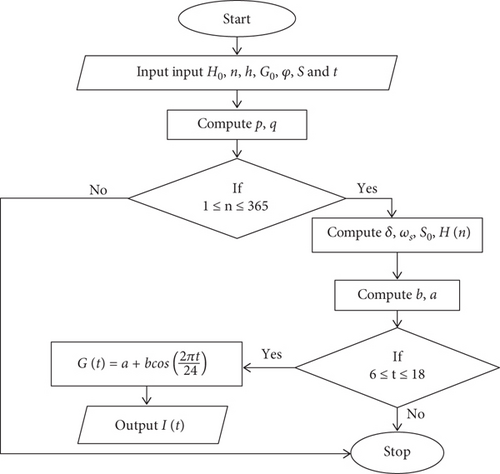
Therefore, the Kaplanis model of Equation (10) becomes completely defined to estimate the irradiance. Figure 2 below shows the Kaplanis model flow chart.

3.2.3. Model 3: Duffie and Beckman Model

The development of the Duffie and Beckman model for Bambili was as follows:

• 1.

  Daylight hours (N):

$$ ()

The sunrise and sunset hours were obtained as the difference between noontime and half-daylight hours as

$$ ()

$$ ()

$$ ()

where ω is the measured solar hour angle in degrees.

• 2.

  The zenith angle (θ_z) and the angle of incidence (θ), measured for the daylight length:

$$ ()

$$ ()

The hourly global solar radiation can be estimated using the equation

$$ ()

Beginning from the rise to the set times of the sun and substituting  cosθ_z, the resulting model below performs as a function of the solar angle.

$$ ()

Replacing ω = 15(12 − t) in the equation, we obtain a model that varies with the solar time.

$$ ()

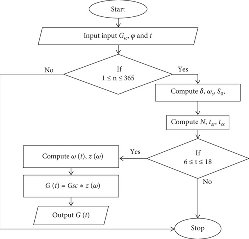
Figure 3 shows the flow chart for the Duffie and Beckman model.

3.2.4. Model 4: Collares-Pereira and Rabl Model

Collares-Pereira and Rabl [16] proposed an irradiance model that was used to obtain irradiance for Bambili as follows:

$$ ()

with G_h representing the average hourly irradiance and G_D representing the average irradiance for the day.

$$ ()

with AST  representing the true solar time. Equation (26) was used for computing true solar time:

$$ ()

where EoT denotes the equation of time, LST represents the local standard time, LSMT is the longitude of the site, and LOD is the local standard meridian time (LSTM) of the location. Just like the Greenwich Mean Time (GMT), which employs the prime meridian, the LSMT is a standard meridian employed for a certain time zone. LSMT is determined as:

$$ ()

Meanwhile, the difference in apparent and mean solar times, measured at a certain longitude at the same real instant of time, results in the  EoT. EoT  can be computed as

$$ ()

where B represents a coefficient measured in degree and can be computed as

$$ ()

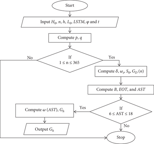
Figure 4 illustrates the flow chart for Collares-Pereira and Rabl.

3.3. Estimation of Temperature Using Different Methods for Bambili

The temperature boundary values of these models were bound by the maximum (T_max) and minimum (T_min) values [23]. The NASA website and AccuWeather provided the T_max and T_min values. For each model, the projected temperatures between dawn and sunset were based on the application of PV systems.

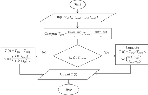
3.3.1. Model 5: WAVE Model

Two intervals were employed with sinusoidal equations to deduce the temperature values, as shown in the following:

For t_sr ≤ t ≤ t_max:

$$ ()

For t_max ≤ t ≤ t_srn:

$$ ()

With

$$ ()

$$ ()

where T(t) is the temperature at hour t,  t_sr is the sunrise time,  t_max is the time the peak temperature occurs (14:00 h), and t_srn is the sunset time. T_ave is the sum mean temperature and T_amp is the difference in mean temperature between the peak and trough temperature values of the day, respectively. The WAVE model with the flow chart shown in Figure 5 required no site-specific calibrations.

3.3.2. Model 6: Parton and Logan (PL) Model

PL’s model makes use of two distinct equations, but we considered only that for daytime applications [24]. It employed a sinusoidal function within the day for estimations. The temperature at any given hour (T(t)) can be calculated based on the photovoltaic system’s operating time as follows:

$$ ()

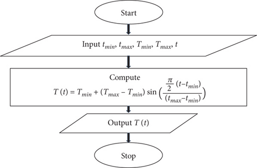
Here,  t_max was 5 h before 6 p.m.

3.3.3. Model 7: SOYGRO Model

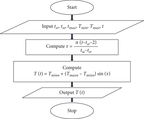
In this model, the daytime equation was used for the estimation of the hourly temperature. In addition to the current day’s T_max and T_min temperature values and based on the operation time of the photovoltaic system, only the daylight hours for estimation from this model were implemented.

Assume,

$$ ()

$$ ()

Figures 6 and 7 show the flow chart for the PL and SOYGRO models.

4. Results and Discussion

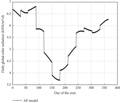
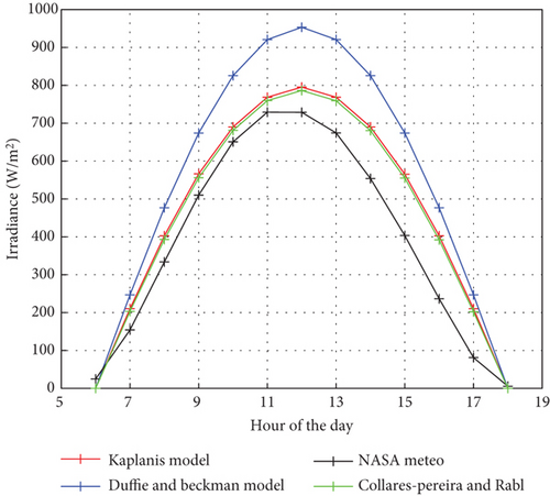
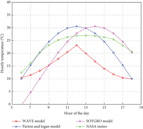
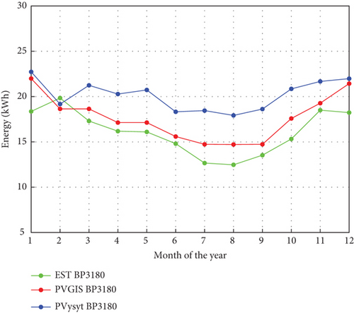
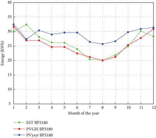
Figure 8 shows the daily global solar radiation in Wh/m²/day for Bambili, Cameroon, using the linear A-P base day of the year model. The results show that the global daily solar radiation (H) for Bambili varies from 4 to 7 Wh/m²/day. The lowest radiation varies between Days 150 and 200, and higher radiation was observed between Days 1 and 100 and between 300 and 365 of the year, which typically is the dry season. Figure 9 shows the plots of the different day-of-the-year models together with the NASA meteorological data. The irradiance obtained with selected models was all above the NASA meteorological website values. This was due to the fact that mathematical models’ maximum values were based on the solar constant with a value of 1000 W/m². This max value turns to drive the predicted values above the NASA meteorological data. The Collares-Pereira and Rabl model shows a lower prediction throughout the day as compared to Kaplanis and Duffie and Beckman models. However, it agrees better with the NASA meteorological data. All the estimation models perfectly agree from sunrise until 9 a.m. and at sunset, with few deviations. Figure 10 shows the plots of the different mathematical temperature models. Unlike the irradiance models, the WAVE model underestimated the temperature throughout the day as compared to NASA temperature data. Figures 11 and 12 show the energy output over the year from the mathematical models and PV online software. Table 2 shows the numerical monthly and annual values of the energy output for Bambili.

5. Conclusions

This work proposed and simulated theoretical models for the estimation of irradiance, temperature, and energy output for Bambili, Cameroon. Methods such as the A-P linear regression model, Duffie and Beckman, Kaplanis, and Collares-Pereira and Rabl models were implemented for estimating the irradiance, while selected methods such as the WAVE, PL, and SOYGRO models were used for temperature estimations. The results obtained from these methods were compared with those obtained from the NASA meteorological database. We deduced that the irradiance prediction for Bambili can be obtained using the Collares-Pereira and Rabl models, while for temperature predictions, the PL models can be employed from 6 a.m. to noon and the SOYGRO model from 1 to 6 p.m.

These estimations can be closer to NASA data if some other parameters are inserted to modify the environmental disturbances, such as sudden cloudiness and rains, among others. With the estimated irradiance and temperature from the selected models, the monthly and annual energy output of solar panels were computed using methods proposed in the literature and PV software. This output ranges from 193.29 to 345.87 kWh. We concluded that for Bambili and other locations without meteorological stations and no internet connections or network service, one can use the day-of-the-year mathematical models to estimate irradiance, temperature, and subsequently the energy output.

Conflicts of Interest

The authors declare no conflicts of interest.

Author Contributions

All authors contributed to the study conception and simulations. Edickson Bobo Yungho and Eustace Mbaka Nfah were responsible for conception, data collection, analysis, and simulations. Tchahou Tchendjeu Achille Ecladore wrote the first draft of the manuscript, and all authors commented on previous versions of the manuscript. All authors were involved in revising the comments given by the editorial board. All authors have read and approved the final manuscript.

Funding

The authors received no specific funding for this work.