The multi-input multioutput (MIMO) systems involving multirelational signals generated from distributed sources have been emerging as the most generalized model in practice. The existing work for characterizing such a MIMO system is to build a corresponding transform tensor, each of whose entries turns out to be the individual z-transform of a discrete-time impulse response sequence. However, when a MIMO system has a global feedback mechanism, which also involves multirelational signals, the aforementioned individual z-transforms of the overall transfer tensor are quite difficult to formulate. Therefore, a new mathematical framework to govern both feedforward and feedback MIMO systems is in crucial demand. In this work, we define the tensor z-transform to characterize a MIMO system involving multirelational signals as a whole rather than the individual entries separately, which is a novel concept for system analysis. To do so, we extend Cauchy’s integral formula and Cauchy’s residue theorem from scalars to arbitrary-dimensional tensors, and then, to apply these new mathematical tools, we establish to undertake the inverse tensor z-transform and approximate the corresponding discrete-time tensor sequences. Our proposed new tensor z-transform in this work can be applied to design digital tensor filters including infinite-impulse-response (IIR) tensor filters (involving global feedback mechanisms) and finite-impulse-response (FIR) tensor filters. Finally, numerical evaluations are presented to demonstrate certain interesting phenomena of the new tensor z-transform.

1. Introduction

Tensors or multidimensional arrays are functions of three or more indices (i, j, k, ⋯), which are mathematical objects generalized from matrices (two-dimensional arrays) and vectors (one-dimensional arrays). The development of new tensor theories and tensor-related algorithms has recently drawn the attention of the signal-processing society [1–3], big-data analytics [4–6], and system design [7, 8] as multirelational characterization among different attributes and objects is crucial for applications of modern signal and system analysis. It is well-known that the z-transform has been applied as an indispensable tool for the analysis and design of discrete-time signals and systems. Generally speaking, the z-transform converts a real- or complex-valued discrete-time sequence to a complex-valued z-function [9–18]. The existing z-transform is actually a scalar function. Recently, the multi-input multioutput (MIMO) systems involving multirelational signals have been emerging as the most generalized model in practice [1–6]. Our preceding work for characterizing such a MIMO system is to build a corresponding “transform tensor,” each of whose entries turns out to be the individual z-transform of a discrete-time impulse response sequence [8]. Take an autoregressive–moving-average (ARMA) tensor-filter for example as illustrated by Figure 1 (the details for implementing an ARMA tensor filter (or a “GARMA” filter) will be presented in Section 5.1 later on). In general, such an ARMA tensor filter involves the “global feedback mechanism” if any of the feedback coefficient tensors

, ⋯,

in Figure 1 is a nondiagonal tensor. A tensor

is a nondiagonal tensor if there exists an entry

such that

(1)

where

. Note that we use semicolons to separate the subscript indices contributed by the row and column parts. The commas between subscript indices are used to separate indices within the same row part or the same column part. For example, the row part of the subscripts of the entry

is i₁, ⋯, i_m while the column part of the subscripts of the entry

is j₁, ⋯, j_m. On the other hand, we say that a MIMO system is without any global feedback mechanism if all feedback-coefficient tensors

, ⋯,

in Figure 1 are diagonal tensors, i.e.,

(2)

where

. If the condition described by Eq. (2) holds, the transfer tensor (refer to [8] for the introduction of transfer tensor) for a MIMO system (the ARMA tensor filter as illustrated by Figure 1) without any global feedback mechanism can be reduced to a tensor whose entries turn out to be the individual rational z-transforms easily as there exists no coupling relationship [8].

Details are in the caption following the image — **Figure 1**
Open in figure viewer PowerPoint

Illustration of the realization of a GARMA-(n, m) filter.

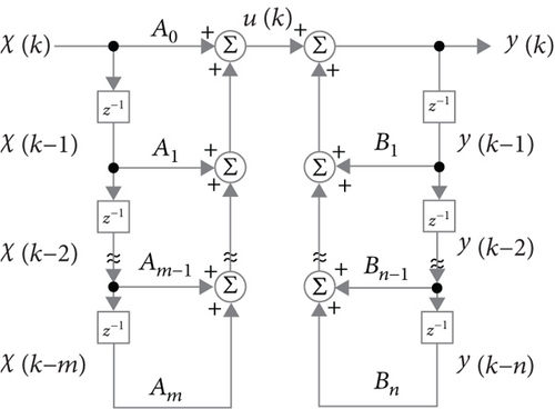
However, when a MIMO system has a global feedback mechanism as described by Eq. (1), which involves the coupling relationship among signals, the aforementioned individual z-transforms of the overall transfer tensor are quite difficult to formulate. Throughout this work, we call a MIMO system without any feedback mechanism a “feedforward MIMO system” where , , ⋯, in Figure 1 are all zero tensors (all their entries are zero); we call a MIMO system without any global feedback mechanism (Eq. (2) holds) a “local-feedback MIMO system” where not all of , , ⋯, in Figure 1 are zero tensors; at last, we call a MIMO system with global feedback mechanism(s) (Eq. (1) holds) a “global-feedback MIMO system.” Therefore, a new mathematical framework to govern all of the feedforward, local-feedback, and global-feedback MIMO systems is in crucial demand. In this work, we propose the novel “tensor z-transform” to characterize an arbitrary MIMO system involving multirelational signals as a whole rather than the individual entries separately.

Some extensions have been made from the conventional z-transform to deal with tensor signals. In [19, 20], the multidimensional z-transformation (referred to as “tensor” in [19, 20]) is introduced to rewrite convolutions and sums of convolutions as products and sums of series. Our proposed tensor z-transform is different from these works since there must involve multiple z-domain variables to characterize a tensor in different ranks in [19, 20]; the multidimensional z-transformation is adopted simply as the generating function for counting the transition probabilities [21] while it is aimed at dealing with the signal and system analysis. To the best of our knowledge, there exists no technique to extend the conventional z-transform from a sequence of complex numbers (scalar) to a sequence of tensors. The obvious difference between the tensor z-transform in this work and the D-transform in [22] is that the tensor z-transform can transform time-domain signals expressed by arbitrary multidimensional arrays (tensors) while the D-transform can only deal with the two-dimensional arrays (matrices). The main difficulty for such an extension is to establish Cauchy’s residue theorem for tensors. In this work, we first define the new tensor z-transform and discuss the related properties. Then, we generalize Cauchy’s residue theorem from scalars to tensors in order to perform the inverse tensor z-transform. Different from the power-series approach, i.e., long division, the time-domain tensor sequence obtained by taking the inverse z-transform via Cauchy’s residue theorem for tensors is not unique since it depends on what contour is chosen in the complex tensor integration. The variability to obtain different time-domain tensor sequences from a tensor z-transform can lead to a new approach to approximate time-domain tensor signal sequences with much less implementational effort from the perspectives of computation and memory complexities. The relationship between the time-domain tensor sequence obtained by applying the power-series approach and that obtained by utilizing Cauchy’s residue theorem for tensors to carry out the inverse tensor z-transform will also be established in this work. An application of tensor z-transform for digital tensor-filter design will be discussed. Besides, the frequency responses of the tensor z-transform, namely, the “ensemble magnitude response” and the “ensemble phase response,” will be investigated. Finally, numerical evaluations will be presented to demonstrate certain interesting phenomena about the tensor z-transform.

The rest of this paper is organized as follows. The concept about tensor z-transform will be introduced in Section 2. New theories regarding Cauchy’s residue theorem for tensors will be presented in Section 3. In Section 4, two approaches to carry out the inverse tensor z-transform, namely, the power-series approach and the integration approach via Cauchy’s residue theorem for tensors, will be introduced. An application of the tensor z-transform for digital tensor-filter design will be presented in Section 5. Numerical evaluations about the frequency responses of the tensor z-transform, the tensor-sequence approximation error, and the implementational complexities will be demonstrated in Section 6. The conclusion will be finally drawn in Section 7.

1.1. Nomenclature

The sets of complex and real numbers are denoted by ℂ and ℝ, respectively. The set of all integers is denoted by ℤ. The natural-number set is represented by ℕ, and ℕ_≥0 denotes the set of nonnegative integers. The symbol “≝” denotes a mathematical definition. The tensor dimensionality discussed in this paper can be expressed by if it is not specified in the context. Note that ι is reserved to represent . Spectrum and eigenvalue share the same meaning throughout this work. Given two invertible tensors , , represents where “⋆_M” denotes the “Einstein product” or “tensor product” as defined in [3].

2. Tensor z-Transform

In this section, we would like to introduce a new mathematical framework, namely, the tensor z-transform. The essential definitions and related examples are presented in Section 2.1 while the important properties are described in Section 2.2.

2.1. Definitions and Examples

A causal tensor sequence

is a tensor sequence such that

for all n < 0 where

denotes an all-zero tensor. The exponential of a tensor

, denoted by

, is written as

(3)

where

and “⋆_M” denotes the Einstein product (a.k.a. tensor product) as introduced in [3]. Consider a sequence of tensors indexed by n, denoted by

where n = 0, 1, 2, ⋯. The tensor z-transform is given by

(4)

Lemma 1 below will establish the required convergence radius of z for Eq.(4). We say a sequence of tensors is a causal tensor sequence if for n < 0, while a sequence of tensors is called an anticausal tensor sequence if for n < 0.

Lemma 1. Consider a power series in terms of the complex variable z as given by

(5)

where

denotes the n-th element (tensor) in a tensor sequence and z₀ denotes an arbitrary complex constant. The radius of convergence of the power series stated by Eq. (5) is thus given by

(6)

where 0 < R < ∞ and “‖ ‖” represents the tensor norm as introduced in [3].

Proof. Without loss of generality, one may assume z₀ = 0. Now we will prove that the power series converges for |z| < R while it diverges for |z| > R instead. Given |z| < R and any ϵ > 0, there exists only a finite number of indices n such that . Consequently, we may have for all but a finite number of tensors , so the tensor series converges if |z| < 1/(1/R + ϵ). Therefore, the power series converges for |z| < R. On the other hand, given ϵ > 0, if we have an infinite number of tensors such that , then |z| = 1/(1/R − ϵ) > R and the tensor series cannot converge since does not converge to 0.

To illustrate the concept of the tensor z-transform, we present the following example.

Example 1. A sequence of tensors is given by where is a constant tensor. Thus, the corresponding radius of convergence is given by

(7)

The z-transform of can be obtained as

(8)

where

denotes an identity tensor (see [3] for its definition). When

is a zero tensor, we have

(9)

where

2.2. Properties

In this subsection, we will introduce several important properties about the tensor z-transform as follows. Due to page limit, we will present the basic properties related to the tensor z-transform, e.g., linearity, time delay, upsampling, and downsampling.

2.2.1. Linearity

Consider a linear combination of two tensor sequences

and

. We have

(10)

where

. According to Eq. (4), we have

(11)

where

and

. Therefore,

(12)

2.2.2. Time Delay

The delayed version

of a tensor sequence

is obtained by delaying k discrete-time instants of

. Thus, we have

(13)

Therefore, we have

(14)

2.2.3. Upsampling

Given a tensor sequence

, we define

, where K ∈ ℕ, by

(15)

for n, i ∈ ℤ. Thus, we have

(16)

Therefore, we have

(17)

2.2.4. Downsampling

Given a tensor sequence

, we define

(18)

Thus, we have

(19)

where the identity “=₁” can be attained according to

(20)

Therefore, we have

(21)

2.2.5. Time Reversal

Given a tensor sequence

, we define

(22)

Thus, we have

(23)

Therefore, we have

(24)

2.2.6. Scaling in the z-Domain

Consider a tensor sequence

where the tensor

is invertible and commutative for

with respect to all n. Thus, we have

(25)

Therefore, we have

(26)

2.2.7. Complex Conjugation

Given a tensor sequence

denotes its complex-conjugated tensor sequence where all elements in

are the complex conjugates of the corresponding elements in

for all n ∈ ℤ. Thus, we have

(27)

Therefore, we have

(28)

2.2.8. Differentiation

Consider a tensor sequence

. Thus, we have

(29)

Therefore, we have

(30)

2.2.9. Convolution

Consider two tensor sequences

and

for n ∈ ℤ, the convolutional tensor sequence

such that

where “⊗_M” denotes the linear convolution operator and

. Thus, we have

(31)

Therefore, we have

(32)

2.2.10. Accumulation

Consider a tensor sequence

where

(33)

Then, we have

(34)

where the identity “=₁” above can be obtained according to the time delay property. Therefore, we

(35)

2.2.11. Initial Value Theorem

According to the z-transform definition given by Eq. (4), we have

(36)

where

is a causal tensor sequence. Taking z⟶∞ at both sides of Eq. (36), we have z⁻ⁿ⟶0. Thus, we have

(37)

2.2.12. Final Value Theorem

According to the z-transform definition given by Eq. (4), we have

(38)

where

is a causal tensor sequence. Thus, we have

(39)

Taking z⟶1 at both sides of Eq. (39), we have

(40)

Therefore, we have

(41)

3. Cauchy’s Residue Theorem for Tensor Sequences

It is well-known that the scalar sequence resulting from the inverse z-transform can be determined using Cauchy’s residue theorem [23]. We will extend Cauchy’s residue theorem to accommodate tensor sequences in this section.

Let us begin with Cauchy’s integral formula for tensors in the following subsection.

3.1. Cauchy’s Integral Formula for Tensors

Let

be a tensor where

(42)

Note that

(43)

λ_k denotes the k-th eigenvalue of

;

and

denote the k-th left and right eigentensors (the definitions of left and right eigentensors can be found in [24]) corresponding to λ_k, respectively; and

is the Hermitian adjoint (the Hermitian adjoint of a tensor is defined in [3]) of

. As we assume that all tensors discussed in this paper are diagonalizable square tensors, all tensors throughout this paper can be expressed in the form of Eq. (42). Furthermore, note that

(44)

where 〈,〉 denotes the inner product of two tensors whose definition can be found in [3];

if k ≠ j while

if k = j;

denotes an identity.

Now define

by the set of all eigenvalues of

, i.e.,

. If f : ♦⟶f(♦) is a function-mapping, where the argument “♦” can be treated as a scalar, vector, matrix, or a tensor, we can formulate

(45)

Let

represent a subset of

. If

only depends on

, we may write

such that

(46)

We further define the functional norm of

(47)

If |f(λ_k)| is bounded for all k, then

. Motivated from [25], we may define the “resolvent”

with respect to a complex variable

such that

(48)

According to Eq. (47), we have

(49)

Lemma 2 below provides the alternative expression of .

Lemma 2. Given a tensor along with its resolvent , we have

(50)

Proof. Since we can express by

(51)

we have

(52)

According to Eq. (52), we can derive Eq. (50).

Lemma 3 below shows that the resolvent is an analytic tensor-valued function of z.

Lemma 3. Given a tensor along with its resolvent , if we have

(53)

then

is an analytic function of z.

Proof. To show that the tensor-valued function is an analytic function of z, we can express by a convergent power series. According to Lemma 2, we can express Eq. (50) by

(54)

subject to

. If we assume that |−z₀| < r, then

(55)

where

. If the condition given by Eq. (53) holds, then

as n⟶∞.

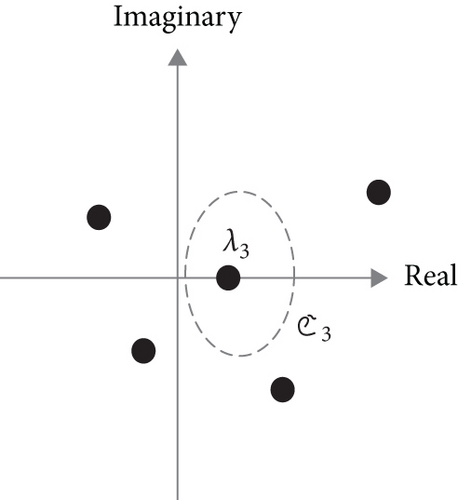
According to Lemma 3, since the resolvent of is analytic, we can carry out the contour integrals over it. For example, a contour ℭ₃ encircles a single eigenvalue, say λ₃, in Figure 2(a) such that

(56)

where the identity “=₁” above follows from

Now we can present Theorem 4 about Cauchy’s integral formula for tensors.

Theorem 4. Given a tensor and an analytic function f(z) with the region of convergence (ROC) including , let be a contour where the set of points are all inside .

Thus, we have

(57)

where is defined by Eq. (46).

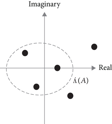
Proof. Consider a contour as illustrated by Figure 2(a) or 2(b). Thus, we have

(58)

Because f(z) is an analytic function with the ROC including , according to the spectral mapping theorem in [25] and Cauchy’s integral formula for scalars in [23], we have

(59)

Define the n-th derivative with respect to the tensor by

(60)

for n = 1, 2, ⋯, where

and “‖ ‖” is the tensor norm as introduced in [3]. Corollary 5 below, which is derived from Theorem 4, presents Cauchy’s integral formula for the “tensor derivatives” given by Eq. (60).

Corollary 5. Given a tensor together with an analytic function f(z) of z with the ROC including . Since is a contour where the set of points are all inside , we have

(61)

for n = 0, 1, 2, ⋯.

Proof. For n = 1 (the first-order derivative), we have

(62)

where “=₁” above is deduced from Theorem 4 and Eq. (60). Thus, Corollary 5 can be established by iterating Eq. (62) repeatedly for n times.

3.2. Generalized Cauchy’s Residue Theorem for Tensor Sequences

is an analytic tensor-valued function with the argument

except for an isolated singularity point at

, then

has a Laurent series such that

(63)

where the coefficient tensor

is called the “residue” of

, denoted by

. Let us present the following lemmas about the residue properties for analytic tensor-valued functions.

Lemma 6. If has a simple pole at and can be expressed by

(64)

where both

and

are analytic at

such that

and

has a simple zero at

, then

(65)

Proof. Since we have

(66)

the identity “=₁” in Eq. (65) can be obtained by multiplying

at both sides of Eq. (66). The identity “=₂” in Eq. (65) can be obtained by

(67)

Lemma 7. If has a pole at with a multiplicity k ∈ ℕ, then we have

(68)

Proof. We have

(69)

Assume . We get

(70)

Thus, according to Eq. (63), Lemma 7 is proven.

Lemma 8 below governs the contour integral of the powers of .

Lemma 8. We get

(71)

for n ∈ ℕ_≥0 and any closed contour ℭ. Moreover, we also have

(72)

for n ∈ ℤ and n < −1.

Proof. For n ∈ ℤ and n ≥ 0, since we have

(73)

Eq. (71) is valid by the binomial expansion of . For n ∈ ℤ and n < −1, since we have

(74)

according to Corollary 5, we get

(75)

Consequently, Lemma 8 is proven.

Now we present Cauchy’s residue theorem for tensor sequences as Theorem 9 below.

Theorem 9 (Cauchy’s residue theorem for tensor sequences). If ℭ is a simple closed contour in the complex z-plane and f(z) is an analytic function with the tensor coefficients except for some tensors with the corresponding spectra , , …, inside the contour ℭ, then we have

(76)

Proof. Assume that m = 1 and is a simple pole. Thus, we can express f(z) by

(77)

where g(z) is given by

(78)

and

denotes the coefficient tensor associated with

for i = 0, 1, 2, ⋯. Besides, we have

By integrating both sides of the following identity:

(79)

we have

(80)

According to Theorem 4 and Lemma 8, we have

(81)

In general, let be an ROC in the complex z-plane containing a contour ℭ and be a subregion of without any of the spectra , , . Consider that these spectra (poles) , , are inside the contours (say small circles) ℭ₁, ℭ₂, …, ℭ_m, respectively, such that ℭ − (ℭ₁ + ℭ₂+⋯+ℭ_m) is inside where “-” and “+” here specify the set difference and union operators, respectively. Theorem 9 is thus proven by applying Theorem 4 and Lemma 8 subject to in both Eqs. (57) and (72). The residue tensors , k = 1, 2, …, m, can be obtained using Lemma 6 if is a simple pole or Lemma 7 if has a multiplicity larger than one.

4. Inverse Tensor z-Transform

In this section, we will introduce two approaches to undertake the inverse tensor z-transform. First, the power-series approach (or long-division approach) will be introduced in Section 4.1 while the contour-integral approach based on our newly derived Cauchy’s residue theorem for tensor sequences will be presented in Section 4.2.

4.1. Power-Series (Long-Division) Approach

Suppose that a tensor z-transform

is expressed by the following rational (proper fraction) form:

(82)

where we assume that m < n without loss of generality (if m ≥ n, we can rewrite Eq. (82) as

, where m^′ < n and

denotes a polynomial of z⁻¹). Given a set of invertible tensors, say

where

for all k, we want to show that it is always possible to find n tensors

, i = 1, 2, ⋯, n satisfying

(83)

Lemma 10. Given where for all k, we have

(84)

solutions totally based on Eq. (83).

Proof. According to the right-hand side of Eq. (83), we have

(85)

According to Chapter 3 in [26], the solution space of ’s in Eq. (83) is equivalent to the solution space of the tensor satisfying

(86)

According to Section 2.2 in [24], the tensors ’s and all can be “unfolded” to form the corresponding υ × υ unfolded matrices, say B_i’s and Z. The solution space of in Eq. (86) is identical to the solution space of Z in the following:

(87)

where O denotes an all-zero matrix. According to Theorem 4 in [27], there are

(88)

solutions of such in Eq. (86). If we know the solution of , i = 1, 2, …, n − 1, to Eq. (87), then Eq. (83) becomes

(89)

where

, i = 1, 2, …, n − 1. Thus, by repeatedly applying Theorem 4 in [27] again and again, there are

(90)

solutions of

’s to Eq. (89). Finally, we will have

(91)

solutions of

for i = 1, 2, …, n, to Eq. (83).

Suppose that we have the following tensor-root decomposition for the denominator polynomial in Eq. (82):

(92)

Consequently, the rational tensor z-function given by Eq. (82) can be expressed by

(93)

where

(associated with the multiplicity κ_i), i = 1, 2, …, ρ, are ρ-distinct roots (in terms of tensors) of the polynomial with tensor coefficients:

. We call the expansion given by Eq. (93) “tensor partial fraction decomposition (T-PDF).” Note that the coefficient tensors

for j = 1, 2, …, κ_i and i = 1, 2, …, ρ in Eq. (93) can be determined using Lemmas 6 and 7 by substituting

for

such that

(94)

where ℓ = 0, 1, …, κ_i − 1 and i = 1, 2, …, ρ.

Furthermore, we can rewrite Eq. (93) to split into the causal and anticausal parts as the following

(95)

where i_c and i_a represent the indices for the causal and anticausal parts of

with ρ_c- and ρ_a-distinct roots (in terms of tensors), respectively, and ρ_c + ρ_a = ρ. Then, the ROC of the tensor z-transform

given by Eq. (95), denoted by

, can be written as

(96)

where

and

denote the set of eigenvalues of the pole tensors

and

, respectively. Because the power-series approach has to consider all pole tensors, one needs to involve all eigenvalues of each pole tensor for determining

. Given a rational tensor z-function

with the ROC specified by Eq. (96), we can find the corresponding inverse tensor z-transform using the power-series (long-division) approach such that

(97)

An example to illustrate how to apply the power-series approach, i.e., long division, to carry out the inverse tensor z-transform is presented below.

Example 2. Here, we will present an example to illustrate how to apply the power-series approach, i.e., long division, to carry out the inverse tensor z-transform. Suppose that is a rational tensor z-function, which can be expressed by

(98)

where

and

denote the numerator and denominator polynomials of the variable z⁻¹, respectively, such that

(99)

(100)

According to Eq. (93), we can express by

(101)

Note that we can obtain the coefficient tensors , and as given by Eq. (94) such that

(102)

According to the power-series approach to undertake the inverse tensor z-transform, we have

(103)

where

(104)

represents the unit-step function with the discrete-time index k and the tensor

is given by

(105)

Thus, according to the power-series method, we have

(106)

Again, according to the power-series approach to undertake the inverse tensor z-transform, we have

(107)

where the tensor

is given by

(108)

Finally, by the linearity of the z-transform, we have

(109)

where and are given by Eqs. (105) and (108), respectively.

Because the eigenvalues of the tensor are 1/2, 1/2, 1/3, and 1/3 while the eigenvalues of the tensor are 1, 1, 1/2, and 1/2, we can determine according to Eq. (96) such that

(110)

4.2. Generalized Contour-Integral Approach

Given an analytic function

and a contour ℭ, according to Theorem 4, we have

(111)

where “=₁” is induced from Theorem 9, ℭ is a simple closed contour in the complex plane, and

is analytic except for the positions at the pole tensors:

, …,

with their corresponding spectra:

for j = 1, 2, …, J_k and k = 1, 2, …, m inside the contour ℭ. Note that J_k ≤ υ and J_k = υ if the closed contour ℭ includes all spectra

. In addition,

if the contour ℭ does not include all eigenvalues of the pole tensors

for k=1, 2, …, m while

if the contour ℭ does include all eigenvalues of the pole tensors

for k = 1, 2, …, m. Different from the power-series approach (which requires all eigenvalues of all pole tensors to be inside ℭ), we can involve only those eigenvalues of the pole tensors inside ℭ in determining

(some eigenvalues of any pole tensor out of the contour ℭ are allowed) in our proposed new contour-integral approach. In summary, it is possible to have

even though

. Therefore, the so-called inverse tensor z-transform is not unique, or precisely speaking, it is contour ℭ dependent. Theorem 11 below will discuss such a contour-dependence property of the inverse tensor z-transform.

Theorem 11. Let be an analytic function except for the positions at the pole tensors , , …, with the corresponding spectra: for j = 1, 2, …, J_k and k = 1, 2, …, m. We have τ contours; i.e., ℭ_i, i = 1, 2, …, τ, and all pole tensors’ eigenvalues inside ℭ_i are collected as the set such that

(112)

If we assume that

(113)

where

according to Eq. (97) and

according to Eq. (111).

Proof. We select a large contour ℭ_∞ that includes all eigenvalues belonging to . Thus, in extension of the inverse (scalar) z-transform study in Section 3.4.1 of [28], we obtain

(114)

where “=₁” arises from Eq. (112).

Suppose that we want to carry out the inverse tensor z-transform of given by Eq. (95) using the generalized contour-integral approach subject to a closed contour ℭ such that , k = 1, 2, …, m, denote the spectra inside ℭ. If there are J_k eigenvalues included in the spectrum , then the ROC of the tensor z-transform given by Eq. (95), denoted by , can be expressed by

(115)

where

and

are the eigenvalues of the pole tensors

and

, respectively. Note that the numbers of eigenvalues in the spectrum

and the spectrum

are represented by

and

, respectively. Different from the power-series approach stated in Section 4.1, the contour-integral approach here only involves the eigenvalues of all pole tensors inside ℭ.

The inverse tensor z-transform via the contour-integral approach can help us to establish the “generalized Parseval’s relation,” given two tensor-sequences, say and with the corresponding tensor z-transforms as given by

(116)

According to the generalized contour-integral approach stated in this subsection, we have

(117)

Therefore, we establish the generalized Parseval’s relation below for tensor sequences:

(118)

An example to illustrate how to apply the generalized contour-integral approach to undertake the inverse tensor z-transform is presented below.

Example 3. In this example, we will illustrate how to employ the generalized contour-integral approach to undertake the inverse tensor z-transform. A rational tensor z-function is given by

(119)

According to Eq. (119), the eigenvalues and the eigentensors of the pole tensor are given by

(120)

Similarly, the eigenvalues and the eigentensors of the pole tensor are given by

(121)

If we consider the inverse tensor z-transform as a causal tensor-sequence subject to a contour ℭ which is any simple closed curve in the region: |z| > 4, and includes the spectrum {1, 1, 2, 2} of the pole tensor and the spectrum {3, 3, 4, 4} of the pole tensor , we have

(122)

Furthermore, if we consider the inverse tensor z-transform as a causal tensor sequence subject to another contour which is any simple closed curve in the region: 3 < |z| < 4, and includes the spectrum {1, 1, 2, 2} of the pole tensor and a partial spectrum {3, 3} of the pole tensor , we have

(123)

Note that we only involve the eigenvalues 3, 3 here because the contour does not include the eigenvalues 4, 4.

5. Applications of Tensor z-Transform

In this section, we will introduce two applications of our proposed tensor z-transform, namely, “tensor filters.” Tensor filters can be widely adopted to characterize massive MIMO (multi-input multioutput) linear-time-invariant (LTI) systems [29–33].

5.1. Infinite-Impulse-Response (IIR) Tensor Filters

Without loss of generality, we consider a discrete-time MIMO LTI system (filter) characterized by a higher-order difference equation with the coefficient tensors

and

such that

(124)

where

and

denote the discrete-time input tensor sequence and the discrete-time output tensor sequence, respectively. The tensor-based MIMO system formulated by Eq. (124) is actually a “generalized autoregressive (AR) and moving average (MA) filter,” denoted by a GARMA-(n, m) filter, which can accommodate arbitrary-dimensional input and output tensor sequences and thus can have much broader applicability than the conventional (single-dimensional) ARMA filters. When there exists a nonzero coefficient tensor among

’s, we call Eq. (124) an infinite-impulse-response (IIR) tensor filter. When there exists a nonzero coefficient tensor among

’s and all of

’s are all-zero tensors, we call Eq. (124) a finite-impulse-response (FIR) tensor filter. When there exists a nonzero coefficient tensor

and all of

’s are all-zero tensors, we call Eq. (124) a GAR-(n) filter. When there exists a nonzero coefficient tensor

and all of

’s are all-zero tensors, we call Eq. (124) a GMA-(m) filter.

Taking the tensor z-transform of both sides of Eq. (124), we have the “transfer tensor” (the definition of a transfer tensor can be found in [8]) ℌ(z) such that

(125)

Let us define

(126)

Then, the output tensor sequence

is given by

(127)

The block diagram given by Figure 1 illustrates how to realize a GARMA-(n, m) filter.

Now consider a special case of m = n. We can decompose Eq. (125) into the following two equations:

(128)

(129)

Taking the inverse tensor z-transform of both sides of Eqs. (128) and (129), we can get

(130)

(131)

The block diagram illustrated by Figure 3 demonstrates how to implement the aforementioned GARMA-(n, n) filter formulated by Eqs. (130) and (131).

5.2. Finite-Impulse-Response (FIR) Tensor Filters

Given the input tensors

, the output tensors

, and the coefficient tensors

and

, the general formula of the finite-impulse-response (FIR) tensor filter can be written as

(132)

where m specifies the maximum tap number. The filter impulse response for Eq. (132) can thus be given by

(133)

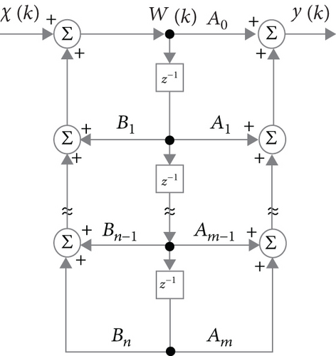
The block diagrams (for the direct forms I and II) illustrated by Figure 4 demonstrate how to implement the aforementioned m-th order FIR tensor filter formulated by Eq. (132).

6. Numerical Evaluation

In this section, we will present the numerical evaluation for an IIR tensor filter. The corresponding frequency and phase responses will be discussed in Section 6.1 while the approximation of discrete-time tensor signals through our proposed spectral-selection technique along with the implementation-complexity analysis will be investigated in Sections 6.2, and Section 6.3, respectively.

Let us consider the following:

(134)

6.1. Frequency and Phase Responses

Given a tensor z-transform

, the frequency response is given by

(135)

where −π ≤ ω < π; ℌ_Re(ω) and ℌ_Im(ω) denote the real and imaginary parts of the frequency response ℌ(e^ιω) (a complex-valued tensor ω-function). If an IIR tensor filter, or a GARMA-(n, m) filter, is realized according to Eq. (125), both ℌ_Re(ω) and ℌ_Im(ω) are real-valued tensor ω-functions. There can be two different definitions about the magnitude response of ℌ(e^ιω). Let us write

. The first is called the “entry-wise magnitude response”

for each entry indexed by i₁, ⋯, i_M; j₁, ⋯, j_M. The second is called the “ensemble magnitude response” ‖ℌ(e^ιω)‖ as defined by

(136)

where “‖ ‖” represents the tensor norm as introduced in [3]. Figure 5 depicts the magnitude responses for the IIR tensor filter characterized by Eq. (134). Two entry-wise magnitude responses

and

are delineated. The ensemble magnitude response ‖ℌ(e^ιω)‖ (denoted by “Ensemble” in the figure) is also delineated in Figure 5. Since the ensemble magnitude response includes the absolute values of all entries according to Eq. (136), it should be larger than any entry-wise magnitude response as illustrated in Figure 5. Besides, we have two definitions for the phase response of the IIR tensor filter having the tensor z-transform

. First, we define the “entry-wise phase spectrum” of ℌ(e^ιω) by

, which represents the phase response of the entry index i₁, ⋯, i_M; j₁, ⋯, j_M. Second, we define the “ensemble phase response” of ℌ(e^ιω) by ∠ℌ(e^ιω) as given by

(137)

where

for all i₁, i₂, …, i_M and j₁, j₂, …, j_M and

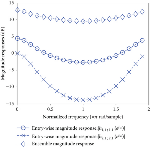
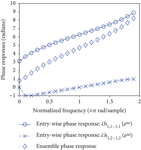
Figure 6 plots the phase responses of the IIR tensor filter characterized by Eq. (134). Two entry-wise phase responses and together with the ensemble phase response, denoted by “Ensemble,” are depicted by Figure 6.

6.2. Approximation of Discrete-Time Tensor Signals via Spectral Selection

According to Section 4.2, we can obtain different inverse tensor z-transforms by selecting different eigenvalues within an integration contour. The norm (the tensor norm is defined in Section 2 of [3]) of the coefficient-tensor at the n-th time index (tap) produced by the inverse tensor z-transform (the transfer tensor) of the IIR tensor filter characterized by Eq. (134) (such that ) is depicted in Figure 7. Let represent the eigenvalues of the pole tensor as highlighted in Eq. (134) enclosed by a contour ℭ selected for the inverse tensor z-transform.

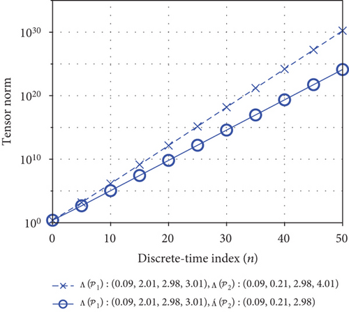
Similarly, let represent the eigenvalues of the pole tensor in Eq. (134) enclosed by a contour C for the inverse tensor z-transform. The red bar-graph in Figure 7 depicts the tensor norms of the inverse tensor z-transform subject to a contour ℭ enclosing the spectra and . Now let us change to and the green bar-graph in Figure 7 depicts the tensor norms of the inverse tensor z-transform subject to a contour ℭ enclosing the spectra and . Note that the tensor norms marked in green are always less than those marked in red with respect to discrete-time indices n since the former tensor norms result from the spectrum of the pole tensor without an eigenvalue 4 in comparison with the latter tensor norms. The legend of Figure 7 denotes the eigenvalues of the two pole tensors and inside a selected contour ℭ.

Given ℌ(z), , and , define the “approximation-error-norm tensor sequence” , where ℭ encloses all eigenvalues of all pole tensors but ℭ^′ leaves out some of them.

Figure 8 depicts the “approximation-error norm” with respect to the discrete-time index n subject to three different contours ℭ^′, where the symbol “⋄” in the figure indicates that ℭ^′ encloses the spectra and , the symbol “°” in the figure indicates that ℭ^′ encloses the spectra and , and the symbol “×” in the figure indicates that ℭ^′ encloses the spectra and .

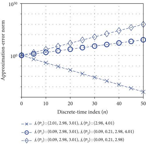
Now we define a “principal eigenvalue” λ such that |λ| > 1 where or . Similarly, we define “minor eigenvalues” λ such that |λ| < 1 where or . According to Figure 8, we observe that the approximation-error norm delineated by the symbol “⋄” is the largest at every k because two repeated principal eigenvalues 2 of the pole tensor and a single principal eigenvalue 4 of the pole tensor are not involved in the contour integral for the inverse tensor z-transform. On the other hand, the approximation-error norm delineated by the symbol “×” is the smallest at every n because all principal eigenvalues (except some minor eigenvalues) of the pole tensors and are involved in the contour integral for the inverse tensor z-transform. As a matter of fact, the approximation-error norm delineated by the symbol “×” will converge to zero as the discrete-time index n approaches ∞. This phenomenon implies the flexibility of our proposed tensor z-transform for the application of approximating an IIR tensor filter characterized by Eq. (125) by another IIR or FIR tensor filter.

6.3. Computational-Complexity Study of Inverse Tensor z-Transform

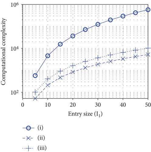
In this subsection, we will investigate the computational complexity for undertaking the inverse tensor z-transform. Suppose

(138)

where and denotes the i-th involved pole tensor with the associated coefficient tensor . If we apply the recursion procedure to carry out Eq. (138), the required computational complexity is given by in terms of the Big-O notation. If we just involve ζ principal eigenvalues inside the contour ℂ to approximate a pole tensor , the required computational complexity is given by since there are υ elements in each eigentensor. Figure 9 depicts the computational complexities required for carrying out Eq. (138) with respect to the entry-size I₁ (note that I₁ = I₂ = ⋯I_M) using the contour-integral subject to the contours enclosing (i) all eigenvalues of all pole tensors (denoted by “○” in the figure), (ii) two eigenvalues of all pole tensors (denoted by “×” in the figure), and (iii) four eigenvalues of all tensors (denoted by “+” in the figure), respectively. The approximation approach can reduce computational complexity significantly according to Figure 9.

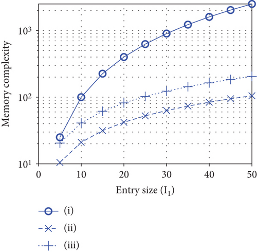
For the memory-complexity study, the exact computation of Eq. (138) requires the memory with the size in terms of the Big-O notation. If we just involve ζ principal eigenvalues inside the contour ℂ to approximate a pole tensor , the required memory complexity is given by since there are υ elements in each eigentensor. Figure 10 depicts the memory complexities required to carry out Eq. (138) with respect to the entry-size I₁ (note that I₁ = I₂ = ⋯I_M) using the contour-integral subject to the contours enclosing (i) all eigenvalues of all pole tensors (denoted by “○” in the figure), (ii) two eigenvalues of all pole tensors (denoted by “×” in the figure), and (iii) four eigenvalues of all tensors (denoted by “+” in the figure). According to both Figures 9 and 10, our approximation approach by use of the contour integral involving fewer eigenvalues of the pole tensors inside a contour can greatly reduce the computational and memory complexities required for the inverse tensor z-transform.

7. Conclusion

In this work, a new arbitrary-dimensional transform, namely, the tensor z-transform, is established to characterize multirelational signals and multi-input multioutput linear-time-invariant systems. The definition of the tensor z-transform is first introduced, and then, the essential mathematical properties are discussed. We extend the conventional Cauchy’s integral formula and Cauchy’s residue theorem for dealing with scalar functions to the new generalized Cauchy’s integral formula and the new generalized Cauchy’s residue theorem for tensor functions. Thus, we propose a new generalized contour-integral approach for undertaking the inverse tensor z-transform. The applications of our proposed new tensor z-transform in this work include the design and approximation of infinite-impulse-response (IIR) and finite-impulse-response (FIR) tensor filters. By selecting the eigenvalues of the pole tensors of a tensor z-transform inside a contour for the inverse tensor z-transform, we can control the corresponding approximation-error norm and the required computational/memory complexity. Our proposed novel tensor z-transform framework can facilitate a promising analysis tool for signal and information processing over networks in the future.

Conflicts of Interest

The authors declare that they have no conflicts of interest.

Acknowledgments

This work was supported by the Louisiana Board of Regents Research Competitiveness Subprogram under Grant LEQSF(2021-22)-RD-A-34.

Open Research

Data Availability

No underlying data was collected or produced in this study.

References

1 Chang S. Y. and Wu H.-C., Tensor Wiener filter, IEEE Transactions on Signal Processing. (2022) 70, 410–422, https://doi.org/10.1109/TSP.2022.3140722.
10.1109/TSP.2022.3140722
Web of Science® Google Scholar
2 Chang S. Y. and Wu H.-C., Tensor quantization: high-dimensional data compression, IEEE Transactions on Circuits and Systems for Video Technology. (2022) 32, no. 8, https://doi.org/10.1109/TCSVT.2022.3145341.
10.1109/TCSVT.2022.3145341
Web of Science® Google Scholar
3 Chang S. Y. and Wu H.-C., Tensor recursive least squares filters for multichannel interrelational signals, IEEE Transactions on Signal and Information Processing over Networks. (2021) 7, 562–577, https://doi.org/10.1109/TSIPN.2021.3110051.
10.1109/TSIPN.2021.3110051
Web of Science® Google Scholar
4 Chang S. Y. and Wu H.-C., Multi-relational data characterization by tensors: tensor inversion, IEEE Transactions on Big Data. (2021) 8, no. 6, 1650–1663, https://doi.org/10.1109/TBDATA.2021.3079265.
10.1109/TBDATA.2021.3079265
Web of Science® Google Scholar
5 Chang S. Y. and Wu H.-C., Tensor kalman filter and its applications, IEEE Transactions on Knowledge and Data Engineering. (2022) 35, no. 6, https://doi.org/10.1109/TKDE.2022.3169129.
10.1109/TKDE.2022.3169129
PubMed Web of Science® Google Scholar
6 Chang S. Y. and Wu H.-C., Multi-relational data characterization by tensors: perturbation analysis, IEEE Transactions on Knowledge and Data Engineering. (2021) 35, no. 1, 756–769, https://doi.org/10.1109/TKDE.2021.3087671.
10.1109/TKDE.2021.3087671
Web of Science® Google Scholar
7 De Lathauwer L., A survey of tensor methods, 2009 IEEE International Symposium on Circuits and Systems, 2009, Taipei, Taiwan, 2773–2776, https://doi.org/10.1109/ISCAS.2009.5118377, 2-s2.0-70350180836.
10.1109/ISCAS.2009.5118377
Google Scholar
8 Chang S. Y. and Wu H.-C., Theoretical and algorithmic study of inverses of arbitrary high-dimensional multi-input multi-output linear time-invariant systems, IEEE Transactions on Circuits and Systems I: Regular Papers. (2023) 70, no. 2, 819–832, https://doi.org/10.1109/TCSI.2022.3217980.
10.1109/TCSI.2022.3217980
Web of Science® Google Scholar
9 Oliaei O., Laplace domain analysis of periodic noise modulation, IEEE Transactions on Circuits and Systems I: Fundamental Theory and Applications. (2003) 50, no. 4, 584–588, https://doi.org/10.1109/TCSI.2003.809804, 2-s2.0-0037936542.
10.1109/TCSI.2003.809804
Web of Science® Google Scholar
10 Das S. and Majhi S., Two-dimensional z-complementary array code sets based on matrices of generating polynomials, IEEE Transactions on Signal Processing. (2020) 68, 5519–5532, https://doi.org/10.1109/TSP.2020.3021986.
10.1109/TSP.2020.3021986
Web of Science® Google Scholar
11 Jaganathan K. and Hassibi B., Reconstruction of signals from their autocorrelation and cross-correlation vectors, with applications to phase retrieval and blind channel estimation, IEEE Transactions on Signal Processing. (2019) 67, no. 11, 2937–2946, https://doi.org/10.1109/TSP.2019.2911254, 2-s2.0-85065396198.
10.1109/TSP.2019.2911254
Web of Science® Google Scholar
12 Das S., Majhi S., Budišin S., and Liu Z., A new construction framework for polyphase complete complementary codes with various lengths, IEEE Transactions on Signal Processing. (2019) 67, no. 10, 2639–2648, https://doi.org/10.1109/TSP.2019.2908137, 2-s2.0-85064677291.
10.1109/TSP.2019.2908137
Web of Science® Google Scholar
13 Verdú-Monedero R. and Gómez-Tornero J.-L., On the use of the z transform of LTI systems for the synthesis of steered beams and nulls in the radiation pattern of leaky-wave antenna arrays, IEEE Transactions on Signal Processing. (2019) 67, no. 9, 2275–2290, https://doi.org/10.1109/TSP.2019.2903992, 2-s2.0-85063864792.
10.1109/TSP.2019.2903992
Web of Science® Google Scholar
14 Chen X., He C., and Peng H., Removal of muscle artifacts from single-channel EEG based on ensemble empirical mode decomposition and multiset canonical correlation analysis, Journal of Applied Mathematics. (2014) 2014, 10, https://doi.org/10.1155/2014/261347, 2-s2.0-84903649888, 261347.
10.1155/2014/261347
Google Scholar
15 Bai R.-F., Li B.-Z., and Cheng Q.-Y., Wigner-Ville distribution associated with the linear canonical transform, Journal of Applied Mathematics. (2012) 2012, 14, https://doi.org/10.1155/2012/740161, 2-s2.0-84864940815, 740161.
10.1155/2012/740161
Google Scholar
16 Al-saleem R. M., Al-Hilali B. M., and Abboud I. K., Mathematical representation of color spaces and its role in communication systems, Journal of Applied Mathematics. (2020) 2020, 7, https://doi.org/10.1155/2020/4640175, 4640175.
10.1155/2020/4640175
Google Scholar
17 Song Y.-E., Zhang X.-Y., Shang C.-H., Bu H.-X., and Wang X.-Y., The Wigner-Ville distribution based on the linear canonical transform and its applications for QFM signal parameters estimation, Journal of Applied Mathematics. (2014) 2014, 8, https://doi.org/10.1155/2014/516457, 2-s2.0-84901809487, 516457.
10.1155/2014/516457
Google Scholar
18 Castillo E., Morales D. P., García A., Martínez-Martí F., Parrilla L., and Palma A. J., Noise suppression in ECG signals through efficient one-step wavelet processing techniques, Journal of Applied Mathematics. (2013) 2013, 13, https://doi.org/10.1155/2013/763903, 2-s2.0-84880147455, 763903.
10.1155/2013/763903
Google Scholar
19 Rovatti R. and Mazzini G., Tensor function analysis of quantized chaotic piecewise-affine pseudo-Markov systems. I. Second-order correlations and self-similarity, IEEE Transactions on Circuits and Systems I: Fundamental Theory and Applications. (2002) 49, no. 2, 137–149, https://doi.org/10.1109/81.983862, 2-s2.0-0036475889.
10.1109/81.983862
Google Scholar
20 Rovatti R. and Mazzini G., Tensor function analysis of quantized chaotic piecewise-affine pseudo-Markov systems. II. Higher order correlations and self-similarity, IEEE Transactions on Circuits and Systems I: Fundamental Theory and Applications. (2002) 49, no. 2, 150–162, https://doi.org/10.1109/81.983863, 2-s2.0-0036475029.
10.1109/81.983863
Google Scholar
21 Mazzini G., Setti G., and Rovatti R., Multimode time-Markov systems: recursive tensor-based analysis, chaotic generation, locally looping processes, International Journal of Bifurcation and Chaos. (2006) 16, no. 4, 961–988, https://doi.org/10.1142/S0218127406015234, 2-s2.0-33745304798.
10.1142/S0218127406015234
Web of Science® Google Scholar
22 Duel-Hallen A., Equalizers for multiple input/multiple output channels and PAM systems with cyclostationary input sequences, IEEE Journal on Selected Areas in Communications. (1992) 10, no. 3, 630–639, https://doi.org/10.1109/49.127784, 2-s2.0-0026844084.
10.1109/49.127784
Web of Science® Google Scholar
23 Oppenheim A. V., Buck J. R., and Schafer R. W., Discrete-Time Signal Processing, 2001, Pearson Education, India.
Google Scholar
24 Liang M. and Zheng B., Further results on Moore-Penrose inverses of tensors with application to tensor nearness problems, Computers and Mathematics with Applications. (2019) 77, no. 5, 1282–1293, https://doi.org/10.1016/j.camwa.2018.11.001, 2-s2.0-85057817960.
10.1016/j.camwa.2018.11.001
Web of Science® Google Scholar
25 Kato T., Perturbation Theory for Linear Operators vol. 132, 2013, Springer Science & Business Media.
Google Scholar
26 Vinberg E. B., A course in algebra, 2003, American Mathematical Soc.
10.1090/gsm/056
Web of Science® Google Scholar
27 Bourgeois G., Nonsymmetric generic matrix equations, Linear Algebra and its Applications. (2015) 476, 159–183, https://doi.org/10.1016/j.laa.2015.03.008, 2-s2.0-84925628725.
10.1016/j.laa.2015.03.008
Web of Science® Google Scholar
28 Proakis J. G., Digital signal processing: principles, algorithms, and applications, 2001, Pearson Education India.
Google Scholar
29 Chen Y.-T., Sun W.-C., Cheng C.-C., Tsai T.-L., Ueng Y.-L., and Yang C.-H., An integrated message-passing detector and decoder for polar-coded massive MU-MIMO systems, IEEE Transactions on Circuits and Systems I: Regular Papers. (2018) 66, no. 3, 1205–1218, https://doi.org/10.1109/TCSI.2018.2879860, 2-s2.0-85057863861.
10.1109/TCSI.2018.2879860
Web of Science® Google Scholar
30 Mahdavi M., Edfors O., Öwall V., and Liu L., Angular-domain massive MIMO detection: algorithm, implementation, and design tradeoffs, IEEE Transactions on Circuits and Systems I: Regular Papers. (2020) 67, no. 6, 1948–1961, https://doi.org/10.1109/TCSI.2020.2968408.
10.1109/TCSI.2020.2968408
Web of Science® Google Scholar
31 Zhang C., Wu Z., Studer C., Zhang Z., and You X., Efficient soft-output Gauss–Seidel data detector for massive MIMO systems, IEEE Transactions on Circuits and Systems I: Regular Papers. (2018) 68, no. 12, 5049–5060, https://doi.org/10.1109/TCSI.2018.2875741, 2-s2.0-85055715383.
10.1109/TCSI.2018.2875741
Google Scholar
32 Attari M., Ferreira L., Liu L., and Malkowsky S., An application specific vector processor for efficient massive MIMO processing, IEEE Transactions on Circuits and Systems I: Regular Papers. (2022) 69, no. 9, 3804–3815, https://doi.org/10.1109/TCSI.2022.3182483.
10.1109/TCSI.2022.3182483
Web of Science® Google Scholar
33 Liu Y., Liu L., Edfors O., and Öwall V., An area-efficient on-chip memory system for massive MIMO using channel data compression, IEEE Transactions on Circuits and Systems I: Regular Papers. (2019) 66, no. 1, 417–427, https://doi.org/10.1109/TCSI.2018.2859361, 2-s2.0-85052718328.
10.1109/TCSI.2018.2859361
Web of Science® Google Scholar

Citing Literature

All articles

Tensor z-Transform

Abstract

1. Introduction

1.1. Nomenclature

2. Tensor z-Transform

2.1. Definitions and Examples

2.2. Properties

2.2.1. Linearity

2.2.2. Time Delay

2.2.3. Upsampling

2.2.4. Downsampling

2.2.5. Time Reversal

2.2.6. Scaling in the z-Domain

2.2.7. Complex Conjugation

2.2.8. Differentiation

2.2.9. Convolution

2.2.10. Accumulation

2.2.11. Initial Value Theorem

2.2.12. Final Value Theorem

3. Cauchy’s Residue Theorem for Tensor Sequences

3.1. Cauchy’s Integral Formula for Tensors

3.2. Generalized Cauchy’s Residue Theorem for Tensor Sequences

4. Inverse Tensor z-Transform

4.1. Power-Series (Long-Division) Approach

4.2. Generalized Contour-Integral Approach

5. Applications of Tensor z-Transform

5.1. Infinite-Impulse-Response (IIR) Tensor Filters

5.2. Finite-Impulse-Response (FIR) Tensor Filters

6. Numerical Evaluation

6.1. Frequency and Phase Responses

6.2. Approximation of Discrete-Time Tensor Signals via Spectral Selection

6.3. Computational-Complexity Study of Inverse Tensor z-Transform

7. Conclusion

Conflicts of Interest

Acknowledgments

Open Research

Data Availability

References

Citing Literature

Figures

References

Related

Information