Volume 2024, Issue 1 6270350

Research Article

Open Access

On Alpha Power Transformation Generalized Pareto Distribution and Some Properties

Salma Omar Bleed,

Salma Omar Bleed

orcid.org/0000-0002-4410-750X

Department of Statistics , College of Science , Al-Asmarya University , Zliten , Libya

Search for more papers by this author

Rasha Abd-Elwahab Attwa,

Rasha Abd-Elwahab Attwa

orcid.org/0000-0003-3246-1293

Department of Mathematics , Faculty of Science , Zagazig University , Zagazig , Egypt , zu.edu.eg

Search for more papers by this author

Rabeea Farag Meftah Ali,

Rabeea Farag Meftah Ali

Department of Mathematics , Faculty of Science , Zagazig University , Zagazig , Egypt , zu.edu.eg

Search for more papers by this author

Taha Radwan,

Corresponding Author

Taha Radwan

[email protected]

orcid.org/0000-0003-1466-8821

Department of Management Information Systems , College of Business and Economics , Qassim University , Buraydah , Saudi Arabia , qu.edu.sa

Department of Mathematics and Statistics , Faculty of Management Technology and Information Systems , Port Said University , Port Said , Egypt , psu.edu.eg

Search for more papers by this author

Salma Omar Bleed,

Salma Omar Bleed

orcid.org/0000-0002-4410-750X

Department of Statistics , College of Science , Al-Asmarya University , Zliten , Libya

Search for more papers by this author

Rasha Abd-Elwahab Attwa,

Rasha Abd-Elwahab Attwa

orcid.org/0000-0003-3246-1293

Department of Mathematics , Faculty of Science , Zagazig University , Zagazig , Egypt , zu.edu.eg

Search for more papers by this author

Rabeea Farag Meftah Ali,

Rabeea Farag Meftah Ali

Department of Mathematics , Faculty of Science , Zagazig University , Zagazig , Egypt , zu.edu.eg

Search for more papers by this author

Taha Radwan,

Corresponding Author

Taha Radwan

[email protected]

orcid.org/0000-0003-1466-8821

Department of Management Information Systems , College of Business and Economics , Qassim University , Buraydah , Saudi Arabia , qu.edu.sa

Department of Mathematics and Statistics , Faculty of Management Technology and Information Systems , Port Said University , Port Said , Egypt , psu.edu.eg

Search for more papers by this author

First published: 16 August 2024

https://doi.org/10.1155/2024/6270350

Citations: 1

Academic Editor: Aliaa Burqan

Share a link

Email
Wechat
Bluesky

Abstract

Recently, the need to develop statistical distributions has become the most important spot. In this context, we employ the α-power transformation (APT) method to convert the generalized Pareto distribution (GPD) into a new distribution. Some statistical properties of the proposed distribution are being studied, such as moments, arithmetic mean, moment-generating function, random variables, entropy, reliability, and hazard function (HF). In addition, the proposed distribution is compared with the Pareto distribution and some other forms of alpha power distributions, such as the alpha power Pareto (APP) distribution, alpha power Rayleigh (APR) distribution, and the alpha power Lomax (APL) distribution. Finally, we demonstrate the benefits of the proposed distribution through a simulation study and two real data sets. It was found that the results showed the MLE method is reliable, the APTGP distribution is a competitive distribution for the aforementioned data set, and it is a mirror image of the Pareto distribution.

1. Introduction

The use of new standard distributions is now widespread in statistical theory. Typically, new distributions are created by combining existing distributions or adding a new parameter using generators [1]. Mudholkar and Srivastava [2] and Marshall and Olkin [3] developed a methodology for adding a new parameter to existing distributions. Eugene, Lee, and Famoye [4] proposed the concept of beta-generated distributions, where the baseline distribution can be the cumulative distribution function (CDF) of any continuous random variable and the parent distribution is the beta distribution. Jones [5] modified the idea of Eugene, Lee, and Famoye [4] and replaced beta distribution with Kumaraswamy distribution. Alzaatreh, Lee, and Famoye [6] proposed the idea of the T-X family of continuous distributions, in which the probability density function (PDF) of the beta distribution was replaced by the PDF of any continuous random variable, and instead of CDF, a function of CDF satisfying certain conditions was used. Barakat [7] constructed a new distribution family by merging a baseline CDF and its reverse, respectively, after adding and subtracting the same positive location parameter from both. He also showed how many more sorts of statistical data can be described by the proposed family than by many other considered families. Moreover, by combining, Barakat and Khaled [8] proposed a new method for constructing a family of CDFs that contains all the possible types of CDFs and possesses a very broad range of indices of skewness and kurtosis. For more details about this subject of the generation of distribution functions, see Al-Hussaini and Abdel-Hamid [9]. Bleed [10] constructed a new four-parameter Kumaraswamy reciprocal family of distributions, Bleed [11], she proposed a new exponential cumulative hazard method for generating continuous family distributions.

The Pareto distribution is a probability distribution that has many applications and is used in applications of reliability theory because it is one of the failure distributions of stress models in mechanical engineering. Also, it is used to describe the income distribution and the extreme behavior of the value of loss in the economic field. In fields of economics, this distribution (Pareto distribution) was after the economist professor Vilfredo Pareto (1848–1923). The Pareto distribution is α-power transformation (APT) law probability distribution that is used in the description of social, quality control, scientific, geophysical, actuarial, and many other types of observable phenomena. Originally applied to describing the distribution of wealth in a society, it fits the trend that a large portion of wealth is held by a small fraction of the population. There are some forms of the Pareto distribution, such as Pareto’s law of the second type (Lomax’s law), Pearson’s law of the sixth type, Pareto’s law of the third type, Pareto’s law of the fourth type, and generalized Pareto distribution (GPD) [12]. Let X is a random variable with Pareto distribution, then the PDF is defined as follows:

( )

where θ is the shape parameter and λ is the scale parameter. If X is a random variable with the generalized form of Pareto distribution, then the PDF is defined as follows:

(1)

with CDF.

( )

where θ is the shape parameter and λ is the scale parameter [13]. Mahdavi and Kundu [14] presented a novel procedure for inserting one more parameter into a continuous distribution known as the APT. Additionally, the Pareto distribution has been used by several writers to propose new classes and research statistical theory. For instance, the GPD was introduced by Pickands [15] to model excess over thresholds instead of maximum. Hosking and Wallis [16] discussed what was estimated using the moments approach (ME). Grimshaw [17] published an approach for calculating the GPD parameters’ maximum likelihood estimation (MLE). Gupta et al. [18] proposed the exponentiated Pareto distribution. Recently, Juárez and Schucany [19] proposed the minimum probability density power divergence method, which allows control over efficiency and robustness. Akinsete, Famoye, and Lee [20] proposed the beta-Pareto distribution. Sarabia and Prieto [21] proposed Pareto’s positive stable distribution to study city size data. Zhang [22] proposed an improved MLE using the empirical Bayesian method. Mahmoudi [23] introduced the beta-GPD. Gómez-Déniz and Calderín-Ojeda [24] developed the ArcTan Pareto distribution and successfully applied it to model insurance data and population size data. de Andrade et al. [25] studied a three-parameter model named the gamma-GPD. The MLE of the GPD for censored data was developed by Pham, Tsokos, and Choi [26]. Ihtisham et al. [27] introduced a new distribution referred to as the alpha-power Pareto (APP) distribution by including an extra parameter. The properties and estimation parameters of the proposed distribution were obtained. The remainder of the paper is organized as follows: In Section 2, we define the new APT generalized Pareto (APTGP) distribution and demonstrate its validity. Section 3 investigates various statistical properties of the APTGP distribution. In Section 4, we compute the Rènyi entropy for the proposed distribution. Section 5 discusses the formulation of reliability and hazard functions (HFs) for the APTGP distribution. Section 6 presents parameter estimation for the APTGP distribution and compares it with other forms of Pareto distributions. Section 7 addresses the goodness of fit test and model selection criteria. In Section 8, we perform a simulation study. Section 9 applies the APTGP distribution to real-life data. Finally, Section 10 provides the conclusion of our findings.

2. APT GPD

Recently, Mahdavi and Kundu [14] proposed a new method called APT. Mahdavi and Kundu [14] defined the PDF and the CDF of the APT method as follows:

( )

Ihtisham et al. [27] introduced the APP distribution with PDFs of the form

( )

where θ is the shape parameter and λ, α are the scale parameters. Therefore, the GPD (1) was transformed into a new one using the APT method, and it is named APT GPD and symbolized by (APTGP). In light of the APT method, the PDF of the APTGP distribution is defined as follows:

( )

Here are θ the shape parameter and λ the scale parameter.

Theorem 1. The function of the new formula for the APT Pareto (APTGP) distribution is a PDF.

Proof 1. The function of the new formula for the APTGP distribution to be a PDF ifff(x) ≥ 0, ∫_xf(x)dx = 1, then

( )

Put,

( )

Therefore, the new formula for the APT Pareto (APTGP) distribution is a PDF. The CDF of the APTGP distribution is defined as follows:

( )

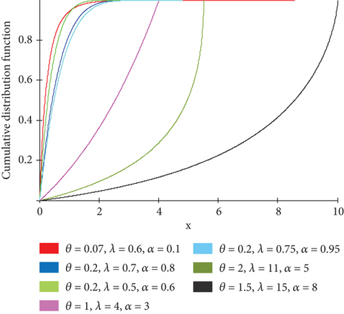
Figure 1 illustrates the CDF of APTGP distribution under different values of the parameters (θ, λ, α), and the plots of the CDF indicate increasing function, concave in shape extending to the right (θ, λ, α > 1), and convex in shape extending to the right (θ, λ, α < 1).

Details are in the caption following the image — **Figure 1**
Open in figure viewer PowerPoint

CDF of APTGP distribution for different values of the parameters.

3. Some Statistical Properties of the APTGP Distribution

Moments: If X is a random variable that follows the APT generalized.

Pareto (APTGP) distribution, then the moments

are defined as follows:

( )

Proof 2.

( )

put

( )

then

( )

Using the series,

( )

Therefore,

( )

(2)

where

and γ(a, b) is the incomplete gamma function.

Arithmetic mean: The arithmetic mean is the first moment, meaning that, put r = 1 in Equation (2); then,

( )

Variance: Variance is the first moment about mean, meaning that, .

Put r = 2 in Equation (2), we get

( )

Therefore, using and , we get

( )

Moment-generating function: Moment generating function of APTGP distribution is defined as follows:

( )

Proof 3.

( )

put

( )

then

( )

Using the series,

( )

Therefore,

( )

Characteristic function: Characteristic function of APTGP distribution is defined as follows:

( )

To generate data x_R from a random variable that follows APTGP distribution, assume that the cumulative function is equal to the random variable U, such that U ~ unif(0, 1). Since F(x) = U, therefore, x_R = λ/θ(1 − A^θ.)

where

( )

Put U = 0.5.

The median is defined as M = (λ/θ)(1 − A^θ), A = (logα²/log(0.5(α − 1) + 1)).

Mode: To find the mode of APTGP distribution, we follow the following steps:

Differentiating the APTGP distribution function for the variable X results in

( )

By equating the differential with zero, we get

( )

Such that f^″(t) < 0

( )

4. Entropy of APTGP Distribution

Rényi entropy of a random variable X with PDF f(x) is a measure of the variation of the uncertainty. For any real parameter, w > 0, w ≠ 1 the Rényi entropy is defined as

( )

Therefore, the Rényi Entropy of APTGP distribution is given by the following:

( )

Let

, then

( )

Therefore, the Rényi entropy of APTGP distribution is given by the following:

( )

Put

( )

Then,

( )

Therefore, the Rényi entropy of APTGP distribution is

( )

5. The Formulation of Reliability and HF

The reliability function (RF) for APTGP distribution can be found as follows:

( )

Figure 2 illustrates the RF of APTGP distribution under different values of the parameters (θ, λ, α), the plots of the RF indicate decreasing RF, convex in shape extending to the right (θ, λ, α > 1), and concave in shape extending to the right (θ, λ, α < 1).

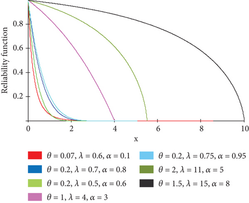
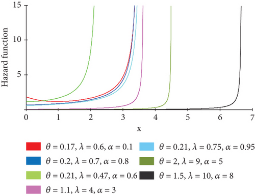
The HF of APTGP distribution can be found as follows:

( )

Figure 3 illustrates the HF of APTGP distribution under different values of the parameters (θ, λ, α), the plots of the HF indicate increasing HF for (θ, λ, α > 1), and for(θ, λ, α < 1).

6. APTGP-Pareto Parameter Estimation

Let X₁, X₂, ⋯, X_n an IID random sample of size n and the order statistics be x₍₁₎ < x₍₂₎ < ⋯<x_(n), then the likelihood and the log-likelihood function of the APTGP Pareto with parameter (α, λ, θ) can be obtained as follows:

(3)

where

is a vector of parameters, that is,

. By taking the log of Equation (3), we obtain

(4)

Therefore, ML estimator

for the unknown parameters (α) will be obtained by solving the following equation numerically.

( )

Now, for obtaining the ML estimators

for the unknown parameters (λ, θ), we assume ω = θ/λ, since 0 < x < λ/θ therefore,

. Therefore, the log-likelihood function (4) can be rewritten as follows:

( )

Therefore, ML estimator

for the unknown parameters (θ) will be obtained by solving the following equation numerically.

( )

Noted that, since , then .

7. Goodness of Fit Test and Model Selection Criterions

This section presents a measurement for model fitting and two model selection criteria. They are as follows.

7.1. Kolmogorov–Smirnov Test

The Kolmokov–Symirnov test (K–S) is used to test whether the data is taken from a population with a specific distribution. It depends on its calculation on the CDF and is one of the distance tests (distance tests). To apply this test, we should arrange the data in ascending or descending order, determine the assumed distribution, and estimate its features. Obtaining the probability value of the cumulative distribution CDF from the specified distribution, and it is denoted by F_n(x_i), and it can be found as follows:

( )

assume that

( )

Then, we calculate the test statistic (KS), which represents the largest distance between D+ and D−, as follows:

( )

7.2. Akaike Information Criterion (AIC)

The AIC used in model testing is generally considered one of the important criteria used in selecting models. This criterion was introduced by Hirotugu Akaike, and this criterion is based on testing models in general for information theory and is defined by the following formula:

( )

such that, lnlf(x|θ_k): The natural logarithm of the maximum likelihood function.

7.3. Modified AIC (MAIC)

MAIC is suggested by Brockwell and Davis [28] by replacing the amount (2 K) with another expression that depends on the principle of correcting the value of AIC and is defined by the following formula:

( )

The model is identical to the data if it has the smallest value of two criteria. In other words, the selection of the matching model depends on the smallest values of (MAIC) and AIC [29].

8. Simulation

The estimation of different simulated APTGP distribution data sets, each with pre-specified parameter values and varying sample sizes, is applied using the Math-Cad program. The ML method to estimate the parameter of the APTGP distribution for eight different simulated random samples of sample sizes ranging from 11 to 400 is applied.

Table 1 presents the estimates of the APTGP parameters along with their mean square error. The results show that the estimates of the parameter are reasonable for all considered random samples of all sizes, and the mean square errors decrease as the sample size increases, which gives an indication that the performance of the ML method is as good as we hope.

Table 1. Results of ML estimators.

n	Estimation of α		Estimation ofθ
n	MLE	MSE	MLE	MSE
Initial values = (α₀ = 1.111, θ₀ = 1.001, λ₀ = 0.884)
11	0.91572	0.0381360	1.00086	0.00000002030
20	1.27495	0.026881	1.00088	0.00000001232
60	1.27342	0.0263814	1.00091	0.00000000797
80	1.25675	0.0212428	1.00096	0.00000000170
150	1.11100	0.0000000	1.00100	0.00000000000
200	1.11100	0.0000000	1.00100	0.00000000000
350	1.11100	0.0000000	1.00100	0.00000000000
400	1.11100	0.0000000	1.00100	0.00000000000
Initial values = (α₀ = 1.12, θ₀ = 1.25, λ₀ = 1.246)
11	0.6778	0.1955	1.3585	0.0118
20	0.912	0.0433	1.3383	0.0078
60	0.954	0.0275	1.3383	0.0078
80	0.985	0.0182	1.3383	0.0078
150	1.0275	0.0086	1.3382	0.0078
200	1.0325	0.0077	1.3383	0.0078
350	1.0361	0.0070	1.3383	0.0078
400	1.042	0.0061	1.3383	0.0078
Initial values = (α₀ = 1.125, θ₀ = 1.25, λ₀ = 1.054)
11	0.7384	0.1495	1.3617	0.0124803851
20	0.9434	0.0329	1.2498	0.0000000266
60	1.0057	0.0142	1.2498	0.0000000230
80	1.0388	0.0074	1.2499	0.0000000080
150	1.0825	0.0018	1.2499	0.0000000070
200	1.0863	0.0015	1.2499	0.0000000060
350	1.0974	0.0008	1.2500	0.0000000003
400	1.1250	0.0000	1.2500	0.0000000000

9. Application to Real-Life Data

To illustrate the importance, usefulness, and flexibility of the APTGP distribution in practice and application, two sets of real industry and medical data were used to compare the APTGP distribution with some other competitive distributions of the Pareto model, such as the Pareto distribution, the APP distribution, the alpha power Rayleigh (APR) distribution, and the alpha power Lomax (APL) distribution. The unknown parameters for the APTGP distribution were estimated using the ML method. The K-S is used to measure the goodness of fit. In addition, AIC, MAIC, and Bayesian IC (BIC) were used to indicate the best-fit distribution of the data. The data fit the probability distribution among the probability distributions that will be referred to later if the null hypothesis is accepted, which states that “the data is fit to the probability distribution, “ and the model with the smallest value of the quality of fit measures will be the best model among them [30].

9.1. Survival Time of Infected With Virulent Tubercle Bacilli

The first data of survival time of infected with virulent tubercle bacilli was reported by [31], which is presented in Table 2.

Table 2. The survival time of infected with virulent tubercle bacilli.

2.16	2.18	2.20	2.20	2.23	2.34	2.41	2.45	2.50	2.59
2.63	2.76	2.86	2.88	2.94	2.94	3.03	3.08	3.10	3.17
3.26	3.51	3.53	3.55	3.64	3.84	3.87	3.89	4.00	4.14
4.16	4.32	4.41	4.52	4.56	4.58	4.58	5.01	5.28	5.89

Table 3 presents the estimates of the APTGP parameters along with their mean square error, and Table 4 shows the suitability of the data for the distribution of APTGP as well as their suitability for the Pareto distribution. This indicates that the APTGP distribution is the best in particular compared to the aforementioned competitive models, as the APTGP distribution gave the smallest value for AIC, MAIC, and BIC compared to the Pareto distribution.

Table 3. ML estimators (survival time of infected with virulent tubercle bacilli).

Distributions		APTGP	Pareto	AP-Pareto	AP-Rayleigh	AP-Lomax
No. of parameters	—	4	2	2	2	3
Initial value	α₀	1.7500	—	1.0090	1.0110	0.0095
Parameter	α	1.7740	—	3.8072	1.0006	0.3067
Mean square error	MSE(α)	0.0006	—	7.8301	0.0001	0.0883
Initial value	θ₀	1.6040	—	0.2500	0.7550	0.0950
Parameter	θ	1.6050	1.6652	1.2006	0.8025	0.2355
Mean square error	MSE(θ)	0.0000	—	0.9036	0.0023	0.0197
Initial value	λ₀	—	—	—	—	0.1870
Parameter	λ	9.4535	1.8121	—	—	0.0960
Mean square error	MSE(λ)	—	—	—	—	0.0083
Parameter	ω	0.1698	—	—	—	—

Table 4. Goodness-of-fit criteria (survival time of infected with virulent tubercle bacilli).

Distributions	K_S^*	L	AIC	MAIC	BIC	Decision
APTGP	0.19713	−65.48006	136.96013	137.62679	142.02676	Fit
Pareto	0.25356	−67.40288	138.80576	139.13008	142.18352	Fit
AP-Pareto	0.44178	−87.50192	179.00384	179.32816	182.3816	Do not fit
AP-Rayleigh	1.6610E + 3	−3.0210E + 8	6.0410E + 8	6.0310E + 8	6.0310E + 8	Do not fit
AP-Lomax	0.66636	−145.93331	297.86662	298.53329	302.93326	Do not fit

^*Critical value at 1% = 0.25773.

Figure 4 demonstrates the graphs of PDF, CDF, reliability, and HFs of the fit distributions. It is noted that the plots of the PDF and the HF of the proposed model APTGP distribution is an increasing function but the PDF of the Pareto distribution is a decreasing function. In addition, the plots of the CDF indicate an increase with decreasing RF of the fit distributions. It has been shown that the RF decreases with the passage of time, meaning that the expected percentages of survival time for those infected with a malignant infection decrease with increasing time, in contrast to the HF, which increases with time.

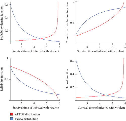
It is noted that the proposed distribution gave a mirror image of the Pareto distribution, and it proved to be a flexible distribution suitable for the data compared to the mentioned distributions.

9.2. Failure Times of the Air Conditioning System of an Airplane

The second data of the air conditioning system of an airplane was originally presented by Linhart and Zucchini [32]. The data is the failure times (weeks) of the air conditioning system of an airplane and is provided in Table 5.

Table 5. The failure times (weeks) of the air conditioning system of an airplane.

0.1250	0.1190	0.1369	0.2500	0.2798	0.3095	0.3690
0.4226	0.4226	0.5179	0.5655	0.5357	0.7143	0.7143

Table 6 presents the estimates of the APTGP parameters along with their mean square error. Table 7 shows the suitability of the data for the APTGP distribution, as well as its suitability for the rest of the distributions, except that it is not suitable for the APP distribution.

Table 6. ML estimators (failure times of the air conditioning system of an airplane).

Distributions		APTGP	Pareto	AP-Pareto	AP-Rayleigh	AP-Lomax
No. of parameters	—	4	2	2	2	3
Initial value	α₀	3.20000	—	10.5000	20.0100	8.05000
Parameter	α	3.20530	—	14.4094	20.0015	12.7779
Mean square error	MSE(α)	0.00003	—	15.2834	0.0001	22.3527
Initial value	θ₀	1.60000	—	0.2000	0.0330	0.9850
Parameter	θ	1.61170	0.9637	0.2943	0.0195	0.9197
Mean square error	MSE(θ)	0.00010	—	0.0089	0.0002	0.0043
Initial value	λ₀	—	—	—	—	0.0650
Parameter	λ	1.15100	0.1190	—	—	0.0997
Mean square error	MSE(λ)	—	—	—	—	0.0012
Parameter	ω	1.38970	—	—	—	—

Table 7. Goodness-of-fit criteria (failure times of the air conditioning system of an airplane).

Distributions	K_S^*	L	AIC	MAIC	BIC	Decision
APTGP	0.06463	2.9876	0.0248	2.4248	1.94197	Fit
Pareto	0.29673	0.75696	2.48607	3.57698	3.76419	Fit
AP-Pareto	-0.06673	-34.91473	73.82947	74.92038	75.10758	Do not fit
AP-Rayleigh	0.05263	−93.1678	190.3356	191.4265	191.61371	Fit
AP-Lomax	0.23963	-4.85036	15.70073	18.10073	17.6179	Fit

^*Critical value at 1% =0.43564.

The APTGP distribution has four parameters compared to the Pareto, Pareto power alpha, and power Rayleigh alpha distributions, which have two parameters, and the three-parameter power Lomax alpha distribution. We noticed that adding these parameters to the new distribution adds features to the distribution, making it more flexible in dealing with aspects of practical life and suitable for life tests.

The results indicated that the distribution of APTGP is the best in particular compared to the aforementioned competitive models, where the distribution of APTGP gave the smallest value for AIC, MAIC, and BIC compared with the rest of the distributions.

Figure 5 demonstrates the graphs of the PDF, CDF, reliability, and HFs of the fit distributions. It is noted that the PDFs of the APTGP distribution are increasing function, but the PDFs of the Pareto, APRD, and APL distributions are decreasing functions. The plots of the CDF indicate an increase with decreasing RF of the fit distributions. It has been shown that the RF for failure times decreases with time, meaning that the expected rates of machine performance decrease with increasing time, in contrast to the HF, which increases with time.

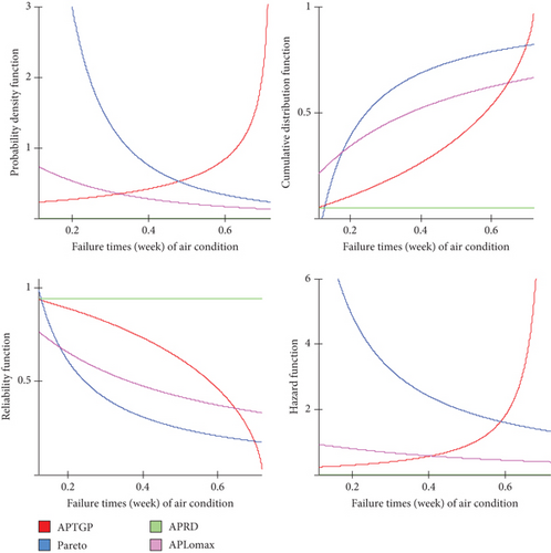
In addition, the plots of the high-frequency distribution show an increasing trend, while those of the Pareto, APRD, and APL distributions exhibit decreasing functions.

10. Conclusion

In this article, a new model called APTGP distribution was proposed, which extends the GPD in the analysis of data with real support. Expansions for the expectation, variance, moments, RF, hazard rate function, moment-generating function, characteristic function, and entropy were derived. The proposed distribution is compared with the Pareto distribution and some other forms of alpha power distributions, such as the APP distribution, the APR distribution, and the APL distribution. Also, the benefit of the proposed distribution is demonstrated through a simulation study and two real data sets. It is clear that the quality of fit values of the APTGP distribution are smaller and closer to the fit of the data than all other distributions, and it is a competitive distribution for the aforementioned data set. Accordingly, the results showed the MLE method is reliable, and the APTGP distribution is a competitive distribution for the aforementioned data set. Also, the APTGP distribution is more flexible than the other distributions, and it will provide greater flexibility in modeling real data because it is a mirror image of the Pareto distribution.

Conflicts of Interest

The authors declare no conflicts of interest.

Funding

The researchers would like to thank the Deanship of Graduate Studies and Scientific Research at Qassim University for financial support (QU-APC-2024-9/1).

Acknowledgments

The researchers would like to thank the Deanship of Graduate Studies and Scientific Research at Qassim University for financial support (QU-APC-2024-9/1).

Open Research

Data Availability Statement

The data presented in this study are available in this article.

References

1 Dey S., Sharma V. K., and Mesfioui M., A new extension of Weibull distribution with application to lifetime data, Annals of Data Science. (2017) 4, no. 1, 31–61, https://doi.org/10.1007/s40745-016-0094-8.
10.1007/s40745-016-0094-8
Google Scholar
2 Mudholkar G. S. and Srivastava D. K., Exponentiated Weibull family for analyzing bathtub failure-rate data, IEEE Transactions on Reliability. (1993) 42, no. 2, 299–302, https://doi.org/10.1109/24.229504, 2-s2.0-0027608675.
10.1109/24.229504
Web of Science® Google Scholar
3 Marshall A. W. and Olkin I., A new method for adding a parameter to a family of distributions with application to the exponential and Weibull families, Biometrika. (1997) 84, no. 3, 641–652, https://doi.org/10.1093/biomet/84.3.641, 2-s2.0-0001324423.
10.1093/biomet/84.3.641
Web of Science® Google Scholar
4 Eugene N., Lee C., and Famoye F., Beta-normal distribution and its applications, Communications in Statistics-Theory and Methods. (2002) 31, no. 4, 497–512, https://doi.org/10.1081/STA-120003130, 2-s2.0-31244433835.
10.1081/STA-120003130
Web of Science® Google Scholar
5 Jones M. C., Kumaraswamy’s distribution: a beta-type distribution with some tractability advantages, Statistical Methodology. (2009) 6, no. 1, 70–81, https://doi.org/10.1016/j.stamet.2008.04.001, 2-s2.0-56949086444.
10.1016/j.stamet.2008.04.001
Google Scholar
6 Alzaatreh A., Lee C., and Famoye F., A new method for generating families of continuous distributions, Metron. (2013) 71, no. 1, 63–79, https://doi.org/10.1007/s40300-013-0007-y, 2-s2.0-84882981547.
10.1007/s40300-013-0007-y
Google Scholar
7 Barakat H. M., A new method for adding two parameters to a family of distributions with application to the normal and exponential families, Statistical Methods & Applications. (2015) 24, no. 3, 359–372, https://doi.org/10.1007/s10260-014-0265-8, 2-s2.0-84944174939.
10.1007/s10260-014-0265-8
Google Scholar
8 Barakat H. M. and Khaled O. M., Toward the establishment of a family of distributions that may fit any dataset, Communications in Statistics-Simulation and Computation. (2017) 46, no. 8, 6129–6143, https://doi.org/10.1080/03610918.2016.1197245, 2-s2.0-85015798442.
10.1080/03610918.2016.1197245
Google Scholar
9 AL-Hussaini E. K. and Abdel-Hamid A. H., Generation of distribution functions: a survey, Journal of Statistics Applications & Probability. (2018) 7, no. 1, 91–103, https://doi.org/10.18576/jsap/070109, 2-s2.0-85061933505.
10.18576/jsap/070109
Google Scholar
10 Bleed S. O., Four parameters Kumaraswamy reciprocal family of distributions, Journal of Data Science. (2019) 18, no. 1, 101–114.
Google Scholar
11 Bleed S. O., New exponential cumulative hazard method for generating continuous family distributions, Journal of Alasmarya University: Basic and Applied Sciences. (2020) 5, no. 1, https://doi.org/10.59743/aujas.v5i1.1646.
10.59743/aujas.v5i1.1646
Google Scholar
12 Pareto V., Cours d′economie politique, Journal of Political Economy. (1898) 6.
Google Scholar
13 Van Montfort M. A. J. and Witter J. V., The generalized Pareto distribution applied to rainfall depths, Hydrological Sciences Journal. (1986) 31, no. 2, 151–162, https://doi.org/10.1080/02626668609491037, 2-s2.0-0022735921.
10.1080/02626668609491037
Web of Science® Google Scholar
14 Mahdavi A. and Kundu D., A new method for generating distributions with an application to exponential distribution, Communications in Statistics-Theory and Methods. (2017) 46, no. 13, 6543–6557, https://doi.org/10.1080/03610926.2015.1130839, 2-s2.0-85014535631.
10.1080/03610926.2015.1130839
Web of Science® Google Scholar
15 Pickands J., Statistical inference using extreme order statistics, The Annals of Statistics. (1975) 3, no. 1, 119–131.
10.1214/aos/1176343003
Web of Science® Google Scholar
16 Hosking J. R. M. and Wallis J. R., Parameter and quantile estimation for the generalized Pareto distribution, Technometrics. (1987) 29, no. 3, 339–349, https://doi.org/10.1080/00401706.1987.10488243, 2-s2.0-0023400777.
10.1080/00401706.1987.10488243
Web of Science® Google Scholar
17 Grimshaw S. D., Computing maximum likelihood estimates for the generalized Pareto distribution, Technometrics. (1993) 35, no. 2, 185–191, https://doi.org/10.1080/00401706.1993.10485040, 2-s2.0-84952103052.
10.1080/00401706.1993.10485040
Web of Science® Google Scholar
18 Gupta R. C., Gupta P. L., and Gupta R. D., Modeling failure time data by Lehman alternatives, Communications in Statistics-Theory and Methods. (1998) 27, no. 4, 887–904, https://doi.org/10.1080/03610929808832134, 2-s2.0-0000865227.
10.1080/03610929808832134
Web of Science® Google Scholar
19 Juárez S. F. and Schucany W. R., Robust and efficient estimation for the generalized Pareto distribution, Extremes. (2004) 7, no. 3, 237–251, https://doi.org/10.1007/s10687-005-6475-6, 2-s2.0-29144515629.
10.1007/s10687-005-6475-6
Google Scholar
20 Akinsete A., Famoye F., and Lee C., The beta-Pareto distribution, Statistics. (2008) 42, no. 6, 547–563, https://doi.org/10.1080/02331880801983876, 2-s2.0-54349094330.
10.1080/02331880801983876
Web of Science® Google Scholar
21 Sarabia J. M. and Prieto F., The Pareto-positive stable distribution: a new descriptive model for city size data, Physica A: Statistical Mechanics and its Applications. (2009) 388, no. 19, 4179–4191, https://doi.org/10.1016/j.physa.2009.06.047, 2-s2.0-67650111619.
10.1016/j.physa.2009.06.047
Web of Science® Google Scholar
22 Zhang J., Improving on estimation for the generalized Pareto distribution, Technometrics. (2010) 52, no. 3, 335–339, https://doi.org/10.1198/TECH.2010.09206, 2-s2.0-77955312065.
10.1198/TECH.2010.09206
Web of Science® Google Scholar
23 Mahmoudi E., The beta generalized Pareto distribution with application to lifetime data, Mathematics and Computers in Simulation. (2011) 81, no. 11, 2414–2430, https://doi.org/10.1016/j.matcom.2011.03.006, 2-s2.0-79959302786.
10.1016/j.matcom.2011.03.006
Web of Science® Google Scholar
24 Gómez-Déniz E. and Calderín-Ojeda E., On the use of the Pareto ArcTan distribution for describing city size in Australia and New Zealand, Physica A: Statistical Mechanics and its Applications. (2015) 436, 821–832, https://doi.org/10.1016/j.physa.2015.02.097, 2-s2.0-84930635724.
10.1016/j.physa.2015.02.097
Google Scholar
25 de Andrade T. A. N., Fernandez L. M. Z., Gomes da Silva F. S., and Cordeiro G. M., The gamma generalized Pareto distribution with applications in survival analysis, International Journal of Statistics and Probability. (2017) 6, no. 3, 141–156, https://doi.org/10.5539/ijsp.v6n3p141.
10.5539/ijsp.v6n3p141
Google Scholar
26 Pham M. H., Tsokos C., and Choi B. J., Maximum likelihood estimation for the generalized Pareto distribution and goodness-of-fit test with censored data, Journal of Modern Applied Statistical Methods. (2018) 17, no. 2, 1–17.
Google Scholar
27 Ihtisham S., Khalil A., Manzoor S., Khan S. A., and Ali A., Alpha-power Pareto distribution: its properties and applications, PLoS One. (2019) 14, no. 6, article e0218027, https://doi.org/10.1371/journal.pone.0218027, 2-s2.0-85067183215, 31188897.
10.1371/journal.pone.0218027
PubMed Web of Science® Google Scholar
28 Brockwell P. J. and Davis R. A., Time series: theory and methods, 1991, Springer science & business media.
10.1007/978-1-4419-0320-4
CAS Google Scholar
29 Akaike H., A new look at the statistical model identification, IEEE Transactions on Automatic Control. (1974) 19, no. 6, 716–723, https://doi.org/10.1109/TAC.1974.1100705, 2-s2.0-0016355478.
10.1109/TAC.1974.1100705
CAS PubMed Web of Science® Google Scholar
30 AlMarzouki S., Jamal F., Chesneau C., and Elgarhy M., Half logistic inverse Lomax distribution with applications, Symmetry. (2021) 13, no. 2, https://doi.org/10.3390/sym13020309.
10.3390/sym13020309
Google Scholar
31 Haq M. A., Kumaraswamy exponentiated inverse Rayleigh distribution, Mathematical Theory and Modeling. (2016) 6, no. 3, 93–104.
Google Scholar
32 Linhart H. and Zucchini W., Model Selection, 1986, John Wiley & Sons.
Google Scholar

Citing Literature

All articles

On Alpha Power Transformation Generalized Pareto Distribution and Some Properties

Abstract

1. Introduction

2. APT GPD

3. Some Statistical Properties of the APTGP Distribution

4. Entropy of APTGP Distribution

5. The Formulation of Reliability and HF

6. APTGP-Pareto Parameter Estimation