Enhancing Smart City Functions through the Mitigation of Electricity Theft in Smart Grids: A Stacked Ensemble Method
Abstract
Smart grid is the primary stakeholder in smart cities integrated with modern technologies as the Internet of Things (IoT), smart healthcare systems, industrial IoT, renewable energy, energy communities, and the 6G network. Smart grids provide bidirectional power and information flow by integrating many IoT devices and software. These advanced IOTs and cyber layers introduced new types of vulnerabilities and could compromise the stability of smart grids. Some anomalous consumers leverage these vulnerabilities, launch theft attacks on the power system, and steal electricity to lower their electricity bills. The recent developments in numerous detection methods have been supported by cutting-edge machine learning (ML) approaches. Even so, these recent developments are practically not robust enough because of the limitations of single ML approaches employed. This research introduced a stacked ensemble method for electricity theft detection (ETD) in a smart grid. The framework detects anomalous consumers in two stages; in the first stage, four powerful classifiers are stacked and detect suspicious activity, and the output of these consumers is fed to a single classifier for the second-stage classification to get better results. Furthermore, we incorporate kernel principal component analysis (KPCA) and localized random affine shadow sampling (LoRAS) for feature engineering and data augmentation. We also perform comparative analysis using adaptive synthesis (ADASYN) and independent component analysis (ICA). The simulation findings reveal that the proposed model outperforms with 97% accuracy, 97% AUC score, and 98% precision.
1. Introduction
With the rapid increase of the world population, conventional cities are becoming overpopulated, which brings forth numerous challenges. A recent United Nations report estimates that the world population will reach 9.7 billion by 2050. Overpopulation faces several challenges such as traffic congestion, energy shortages, lack of a healthcare system, natural resource depletion, and water shortages [1].
Smart cities are the feasible substitutes for traditional cities, which offer promising solutions to mitigate the challenges posed by overpopulation. Smart cities leverage many technological advancements, such as the IoT, smart grid, industrial IoT, smart homes, 6G network, smart health care, renewable energy, and energy community [2], to optimize resource allocation and improve the inhabitants’ quality of life. Figure 1 exhibits a futuristic smart city integrated with many technological advances. The smart grid is one of the primary stakeholders in futuristic smart cities. As the smart grid is arguably the paramount aspect of a smart city, it provides an uninterrupted power supply to the entire system and acts as the soul of a smart city, while, in the event of unavailability of a smart grid for a considerable duration, all other features of the smart city will inevitably be ceased [3].

The emergence of the smart grid with IoT devices introduces many technological advances in the rapid development of smart cities. This enables more advanced and efficient energy systems by integrating cutting-edge communication, monitoring, and control to the conventional power grid architecture. It optimizes energy flow, stabilizes grid structure, supports renewable energy sources, and provides a bidirectional communication among power generation, distribution network, and end consumers. These collective features result in an energy framework that is not only more dependable and sustainable but also resilient. Many countries like China, the USA, Germany, Brazil, and Japan are making many efforts to develop conventional grids into smart grids and use clean energy to power their smart grids [4]. According to a recent report, it is estimated that the USA invests 3.6 billion dollars in the smart meter market in the year 2022. The world’s second-largest economy China is anticipated to reach a projected market size of 15.4 billion by 2030, which captures the compound annual growth rate of 9.4% of the market size by 2022 to 2030. Moreover, Canada and Japan are two more notable regional markets, with growth rates of 6.7 and 5.9, respectively, by the period of 2022–2030 [5]. The smart grid incorporates a variety of IoT devices (e.g., smart meters, sensors, and data centers) and software (e.g., cyber layer). This introduces many security risks, such as cyberphysical attacks and manipulation of communication systems and IoT devices in smart grids. Some suspicious consumers leverage these security risks to launch physical attacks (bypassing smart meters) and cyber theft attacks (injecting false meter readings) to lower their electricity bill [6]. Cyberattacks are more discreet and versatile as compared to physical attacks, as they can be launched remotely from any corner of the world. Moreover, the regions with widespread electricity theft face power quality problems, and more frequently, brownouts and blackouts happen.
These security risks compromise the stability and operation of smart gird. It causes high revenue loss for the country and seriously jeopardizes public safety. According to a recent report, worldwide electricity utilities faced 96 billion dollars of loss annually in 2014 because of electricity theft [7]. As a result, electricity tariff increases for all consumers by passing all economic losses to all honest consumers. Similarly, electricity theft has been affecting other sectors most (e.g., healthcare system and industrial system). In contrast, electricity theft affects uninterrupted power supply to the industrial systems, which causes huge production interruptions and losses of millions of dollars in terms of delays in completing orders for their customers. Moreover, the healthcare system is the most vulnerable and highly affected by electricity theft, which causes interruptions in critical health equipment and life-saving procedures and highly compromises patient care. Furthermore, energy theft is caused by various circumstances, including weak economic situations and high energy tariffs [8]. Therefore, it is necessary to have an electricity theft detection framework to secure the smart grid from malicious consumers. The conventional detection methods, which depend on manual on-site inspection, take a lot of time and money.
Data-oriented methods of electricity theft detection are becoming more popular as smart meters generate huge amounts of electricity consumption data. The data-driven approach uses ML techniques to detect variations in the consumption history and identify abnormal consumption, which highly relates to energy theft. We take electricity consumption data from the State Grid Corporation of China (SGCC) for the evaluation of our proposed system model.
1.1. Contribution
- (1)
The introduced stacked framework amalgamates the inherent perks of two-stage sample analysis, resulting in improved suspicious activity detection, high convergence rate and enhanced the overall efficiency of the smart grid.
- (2)
This research achieves a significant contribution by utilizing KPCA as a powerful nonlinear feature extraction technique to handle the curse of dimensionality in the presence of such a high-dimensional dataset.
- (3)
The class imbalance is a major issue as there is frequent occurrence of theft events. Therefore, we incorporate the LoRAS approach to combat the class distribution issue. The LoRAS technique strategically generates augmented samples, which allows a more accurate and balanced representation of the theft class. It helps the classifier to prevent bias and improve the generalization of the classifier.
- (4)
Furthermore, we perform a comparative analysis by integrating independent component analysis (ICA) and adaptive synthesis (ADASYN) techniques for feature engineering and data augmentation, respectively, on the same framework.
2. State-of-the-Art Work
2.1. Machine Learning-Based ETD
The related work is discussed in detail in Table 1, which identifies the research gaps, proposed solutions, contributions, and existing limitations. To address the issues of theft-based nontechnical losses (NTLs), Reference [9] proposed a pattern-based and context-aware technique for ETD. To compute the chance of malevolent consumers, the suggested technique takes into account the appropriate calendar context and aspects of daily power usage for a specific day. The K-nearest neighbors (K-NN) and dynamic temporal warping (DTW) are used in this technique, with K-NN being used to rank the change from time to time of the given day and DTW being used to accurately record the link between two consumption patterns. This study describes several types of theft attacks and evaluates the viability of the suggested strategy. The findings showed that the suggested technique had a false-positive rate (FPR) of 1.1%, a true-positive rate (TPR) of 93%, and an overall F1 score of 94% all of which support the model’s effectiveness in identifying power theft. These results support the idea that the technique performs better than earlier works in terms of low FPR and high detection rates.
| Research gap | Proposed methodology | Contributions | Limitations |
|---|---|---|---|
| Data security | KNN and DTW [9] | Precision, F1 score, FPR, and TPR | KNN requires high memory for training |
| Cyberphysical attacks | Cumulative sum and Shewhart control chart [10] | FPR and FNR | Insufficient data and performance measures |
| Imitation of power lines | MCC [6] | Accuracy, precision, recall, F1 score, and PR-AUC | Low DR |
| Abnormal power loss detection at feeder level | SVM [11] | DR, FAR | Insufficient data and training complexity of SVM technique |
| Limitations of conventional correlation-sorting methods | Correlation analysis method [12] | AUC score, MAP, and PCC | Less effective in case of multiple theft consumers stealing energy at fix ratio |
| Cybertheft attacks | SMOTE-borderline and ConvLSTM [13] | Accuracy, precision, F1 score, and execution time | Borderline SMOTE ignores normal minority samples on border area |
| Misclassification | CNN-LSTM-BWO [14] | Accuracy, F1 score, and AUC-ROC | SMOTE causes overfitting |
| Low accuracy | DWT and FCM [15] | AUC and MAP | FCM not suitable for large datasets and DWT causes loss of information |
| Low accuracy and DR | Autoencoder and MLHN [16] | Precision, recall, F1 score, and AUD-ROC curve | MLHN can prone to overfitting |
| Low DR and FA | LSTM-SAE [17] | Detection rate, false alarm, and highest difference | Computationally expensive |
| Less proficiency | LSTM and AE [18] | DR and FAR | LSTM require high memory and AE can prone to overfitting |
| Computationally expensive and high execution time | Bayesian optimizer and DNN [19] | Accuracy, F1 score, and AUC-ROC | DNN requires large amount of data for training |
| Curse of dimensionality | GCN and CNN [20] | AUC, MAP@100, and MAP@200 | GCN is vulnerable to over smoothing |
| High dimensionality | CNN_MR [21] | Precision, recall, AUC-PR, and AUC-ROC | Low generalization |
| Class imbalance | DQN [22] | Precision, TPR, FPR, FOR, and F1 score | DQN requires large amount of data for training |
| Cyberattacks | AAE, CR, and FFNN [23] | FNR, DR, and FA | FFNN are prone to overfitting |
| Electricity theft | CAE and Tr-XGBoost [24] | Global error, accuracy of priority order, and recovery rate | Complex system and high computational |
| Privacy issue | FE and FFNN [24] | DR, HD, FAR, and accuracy | Overfitting |
| Low FPR | DNN and PSO [25] | TPR, FPR, AUC-ROC, and BDR | Computationally expensive |
The implicit assumption that malevolent users manipulate smart meter readings to values far lower than their real power consumption hinders the effectiveness of the current electricity theft detection methods. Attacks involving substantial power theft are referred to as large-amount electricity thefts (LETs). However, some malevolent users could be circumspect enough to execute small-amount energy theft (SET), where smart meter readings are changed to numbers only a bit lower than the true values, mostly to avoid detection. In order to overcome this constraint, Reference [10] provides a detector that can successfully counter SET and LET attacks. This detector examines measurements of a central observer meter and reported readings from users using a Shewhart control chart and a cumulative sum (CUSUM) control chart in combination. It comprises an electricity theft detection phase that seeks to promptly identify the existence of LET/SET assaults and a malicious user identification phase that seeks to precisely identify malicious users. The suggested detector has undergone extensive testing, and the findings indicate that it performs well across a number of measures.
However, recent developments are not practical enough, in part because of the weaknesses of the ML algorithms used. Study in [6] proposed a covert power stealing approach for a set of smart houses by simulating typical consumption patterns and simultaneously hacking nearby meters. Existing techniques are nearly unable to identify such an assault since the modified data hardly deviate from accurate use records. First, establish and define two degrees of consumption deviations, interpersonal-level and home-level, to address this issue. Next, develop a feature extraction strategy that can identify the relationship between assaults and loyal clients. Finally, create a fresh detection model based on deep learning. Numerous tests using real-world data demonstrate that the disclosed assault might avoid common mainstream detectors while still generating large profits. Additionally, the suggested countermeasure performs better than cutting-edge detection techniques.
Power loss, which includes both nontechnical and technical loss, represents the effective utilization rate of energy, as well as the management level of power networks. Reference [11] provides a data-driven combination approach for systematically identifying power loss abnormalities in distribution networks (DN), including anomalous position, anomalous kind, and timing. There are three steps to the detection process: abnormal position detection, aberrant feeder detection, and abnormal time detection. The data-driven algorithm based on electricity sales data and daily power supply initially detects probable anomalous feeders from all feeders in DN. The control chart is then used to thoroughly monitor the variation of each anticipated abnormal feeder’s power loss and determine its abnormal time. Numerous real data experiments indicate that the suggested data-driven combination algorithm can detect and evaluate anomalous power loss in DN.
Because stealing tendencies spread among consumers, collaborative energy theft, such as village fraud, has become especially widespread. In [12], a group of electrical thieves who steal energy at a consistent ratio was considered. When several electrical thieves are in the same location, conventional correlation-sorting algorithms may struggle. To circumvent this constraint, we first develop a mathematical model of NTL using load data from fixed ratio electricity thieves (FRETs). Following that, an intriguing correlation pattern was noticed and investigated, which may be used to locate FRETs. Suggest a correlation analysis-based detection approach based on this trend. It uses standardized covariance to assess the relationship between the user data and NTL. FRET detection is accomplished by addressing a combinatorial optimization problem. In practice, a similar framework was also created. Finally, numerical tests using an actual dataset and an electrical theft dataset from an electricity theft emulator (ETE) are carried out to confirm the proposed method’s efficacy and superiority in terms of accuracy, stability, and scalability.
2.2. Deep Learning-Based ETD
Energy theft is difficult to spot in a traditional power infrastructure due to restricted communication and data transfer. The combination of smart meters and big data mining technologies results in substantial technical advancement in the field of ETD. Reference [13] presented an ETD model based on convolutional LSTM to detect electricity theft consumers. Electricity usage data are reshaped quarterly into a 2-D matrix and utilized as the sequential input to the convolutional LSTM. The convolutional NN contained in the LSTM can more effectively learn data characteristics on multiple quarters, days, weeks, and months. Furthermore, the suggested model includes batch normalization. This methodology facilitates the integration of raw-format power consumption data directly into the proposed ETD model, thereby reducing training overhead and improving model deployment efficiency. Results from the case study indicate that the convolutional LSTM model proposed demonstrates robustness, outperforming both multilayer perceptron and CNN-LSTM models in terms of performance metrics and generalization capabilities. Moreover, the findings demonstrate that employing K-fold cross-validation techniques can enhance the accuracy of ETD prediction.
The authors in [14, 26] suggested deep learning algorithms for detecting power theft. A three-stage approach for feature selection, extraction, and classification has been developed. The average hybrid feature significance identifies the most significant traits and high priority throughout the selection process. The feature extraction methodology leverages the ZFNET method to eliminate undesirable features. We used the LSTM approach included in the CNN methodology to identify electric fraud. To generate optimum values for CNN-LSTM hyperparameters, meta-heuristic approaches such as Blue Monkey Optimization (BMO) and Black Widow Optimization (BWO) are utilized. The adjustment of the classifier’s hyperparameters aids in better data training. Following the thorough simulation, our suggested approaches, CNN-LSTM-BMO and CNN-LSTM-BWO, obtained 91% and 93% accuracy, respectively. All of the previous comparable strategies are outperformed by the proposed approaches. The performance of models has achieved great accuracy and a low error rate. However, the integration of the Synthetic Minority Oversampling Technique (SMOTE) causes overfitting and data-bridging effects.
The author in [15] proposed a unique unsupervised data-driven strategy for detecting power theft in AMI. Observer meter data, fuzzy c-means (FCM) clustering, and wavelet-based feature extraction are all used in the process. To distinguish between legitimate and fraudulent users, a new anomaly score is created according to the level of cluster membership information given by FCM clustering. Using a publicly accessible smart meter dataset, we conduct ablation research to assess the influence of key aspects of the proposed technique on performance. The findings reveal that all main components of the suggested technique greatly increase performance. The suggested technique is compared against a collection of baselines, including state-of-the-art methodologies that employ smart meter data from commercial and residential consumers. The comparative findings show that the suggested technique outperforms the baseline methods in terms of detection performance.
The increasing adoption of household smart meters and energy monitoring devices facilitates the collection of extensive data for analyzing residential electricity consumption. These data can be leveraged to enhance the detection of electricity leakage and theft, identify instances of tampering and data fraud, and pinpoint powerline failures. The time window approach is initially presented in [16] to extract the characteristics and potential periodicity of home electrical data. A multilayer hierarchical network (MLHN) is then created to identify anomalies in single sensor data and categorize numerous groups of sensor data, respectively, by combining the denoising capacity of the autoencoder with the induction capability of the feedforward neural network. The experimental findings reveal that as compared to the provided method, the accuracy of identifying aberrant data and data categorization is greatly enhanced.
The existence of malicious, aberrant data packets in a dc microgrid’s cyber layer might impede control objectives, causing voltage instability and changing load dispatch patterns. As a result, recognizing abnormal data is critical for restoring system stability. Reference [17] addresses two critical research questions: (1) Which data-driven detection strategy provides the highest detection performance in dc microgrids against stealth cyberattacks? (2) How does combining two features (current and voltage data) for training increase detection performance when compared to utilizing a single feature (current)? Research found that (1) using an uncontrolled deep recurrent autoencoder anomaly detection technique in dc microgrids outperforms other standards in terms of detection performance. The autoencoder is trained using nonthreatening data supplied by a multisource dc microgrid model. (2) Using current and voltage data together for training results in a 14.7% improvement. The effectiveness of the results is demonstrated using experimental data acquired from a dc microgrid testbed during stealth cyberattacks.
In [18], author proposed using deep (stacked) autoencoders with a sequence-to-sequence (seq2seq) structure based on LSTM. The depth of the autoencoders’ structure aids in capturing intricate data patterns, while the seq2seq LSTM model allows for data exploitation due to its time-series nature. We examine the detection performance of a basic autoencoder, a variational autoencoder, and an autoencoder with attention (AEA), finding that seq2seq structures outperform fully linked ones. Depending on the simulation findings, the AEA detector outperforms existing state-of-the-art detectors by 4–13% and 4–21% in terms of false alarm rate and detection rate, respectively. Reference [27] covered the subject of energy theft and present detection systems, providing insight into future research objectives. After examining how attackers tamper with meter readings, we conduct a comprehensive assessment of all current detection approaches, which are divided into measurement mismatch-based methods and machine learning. Electricity theft’s negative impacts, as well as its political and social implications, are also discussed. The survey can assist relevant academics set future research paths, particularly in the field of creating new effective ways for detecting electricity theft.
The authors in [19] introduced a method for detecting theft that employs extensive characteristics in the time and frequency domains in a deep NN-based classification approach. The authors also addressed dataset shortcomings like missing data and class imbalance via data interpolation and synthetic data generation. We analyzed feature significance across temporal and frequency domains, and conduct experiments in a combined, PCA-reduced feature space. Furthermore, a minimal redundancy maximum relevance technique is applied to validate key features that enhanced power theft detection performance by tuning hyperparameters with a Bayesian optimizer and utilizing an adaptive moment estimation (Adam) optimizer to test various critical parameter values for optimal configuration. Finally, it demonstrates the proposed method’s competitiveness in contrast to other approaches assessed using the same dataset. Proposed methods acquired 97% area under the curve (AUC), which is 1% better than the best AUC in previous research, and 91.8% accuracy, which represents the second highest on the benchmark.
The broad use of modern metering infrastructure provides a chance to identify power theft by evaluating data obtained from smart meters. Existing models, however, perform poorly in detecting power theft because most of them are unable to recognize the time dependency, periodicity, and latent features from complicated electrical consumption data. In [20], a Graph CNN and an Euclidean CNN are coupled to produce a unique model for detecting power theft. On the one hand, a novel approach to graph theory is used to describe the high-dimensional power demand curves as a graph. Next, the GCN performs graph convolutional operations to represent the time dependency and periodicity. On the other hand, CNN uses Euclidean convolutional techniques to extract the latent characteristics from the power load curves. Numerical simulations demonstrate that the suggested model outperforms the industry standards in detecting energy theft by combining the advantages of GCN and CNN.
Several cutting-edge ETD approaches are investigated, and their advantages and disadvantages are analyzed in [28] in a thorough overview. Modern ETD approaches are categorized using three levels of taxonomy. Different energy theft methods and their effects are examined and summarized, and various performance metrics to compare the effectiveness of suggested tactics are taken from the literature. Future research is advised to address the difficulties presented by various ETD approaches and their mitigation. It has been noted that the work on ETD lacks knowledge management strategies that might improve both ETD and theft tracking. Both for ETD and future energy theft prevention, this can be helpful.
Electromechanical and digital power meters coexist with smart meters, presenting challenges in monitoring NTL and fraud. Traditional electromechanical meters, read monthly by operators, contrast with smart meters that provide high-resolution power readings. Sampling frequencies vary, with some customers’ usage recorded every 15 minutes and others monthly. Given the extensive historical monthly consumption data already held by businesses, leveraging these data for predictive analytics could enhance NTL management on smart grids. In order to concurrently train and forecast input consumption curves collected once per month or every 15 minutes, Reference [21] proposed a multiresolution deep learning architecture. The suggested algorithms are examined using a sizable data collection of consumers, both with and without fraudulent actions, gathered from the Uruguayan utility company UTE and a public access dataset with artificial fraud. Results demonstrate that the multiresolution architecture outperforms methods developed for a certain class of meters.
Energy theft-related electrical loss, also known as NTL, is one of the issues with the electricity grid system. The unanticipated electrical losses put the grid system’s stability and sustainability in threat. One way to address the issues with NTL is through the identification of energy theft through data analysis. The unequal class dataset of collected power use is the key issue with data-based NTL identification. To address the data unbalanced problem of NTL, deep reinforcement learning (DRL) is used in [22] to approach the NTL detection problem. The suggested technique’s benefit is that it uses the classification method to employ incomplete input features rather than using a preprocessing method to choose input features. Moreover, as compared to typical NTL detection methods, additional preprocessing procedures to maintain the dataset are not required. According to the simulation findings, the suggested technique outperforms traditional methods in a variety of simulation scenarios.
The smart grid is increasingly concerned about electricity theft. Using energy by electric utilities without an agreement and manipulating meter readings to reduce or avoid paying the electricity bill are examples of unauthorized consumers using energy. Significant research has been done in the past ten years to stop and fight stealing. A basic summary of the development of power theft detection, comprising threat models, datasets and input features employed, procedures and approaches, and assessment metrics, is provided in [29] and compared the effectiveness of each detection method as well.
The authors in [23] examined how well power theft detectors defend themselves from evasion assaults. By inserting adversarial samples, such assaults lower the reported electricity reading levels and trick the power theft detectors. Repeatedly creating adversarial samples based on an electrical reading and its nearby readings suggests significant evasion techniques that trick the benchmark detectors. Depending on the attacker’s knowledge of the detector’s parameters or datasets, we use white-box, gray-box, and black-box settings to analyze the effects of evasion assaults. According to the proposed research, the performance of benchmark detectors can degrade in white-, gray-, and black-box conditions by up to 35.8%, 26.9%, and 22.2%, respectively. Successively merging a convolutional-recurrent, attentive autoencoder, and feedforward NNs presents an ensemble learning-based anomaly detector to identify undetected assaults (traditional and evasion), which is trained entirely on benign data. The suggested model provides steady detection performance with maximal adversarial sample injection levels, with average degradation being just 0.7–3%, 0.9–2.1%, and 0.4–1.7% in white-, gray-, and black-box conditions, respectively.
A two-step technique for detecting energy theft is introduced in [24] to locate electricity theft users and forecast probable stolen electricity (PSE) in order to maximize financial gain. The convolutional layer is used in the convolutional autoencoder (CAE), a neural network model, in the first stage to extract and recognize the anomalies of electricity fraud users against the regularity and periodicity of typical power consumption parameters. The Tr-XGBoost technique, a fusion of the Extreme Gradient Boosting (XGBoost) algorithm and the Transfer Adaptive Boosting (TrAdaBoost) training method, is applied in the second stage for predicting the probable suspected electricity (PSE) of each detected power theft user. Tr-XGBoost establishes the relationship between the extracted electricity characteristics and the PSE of each fraudulent electricity user. Based on the predicted PSE, a selection of electricity theft users for investigation is made to maximize economic return. Case studies conducted on the IEEE 33-bus test system and a low-voltage distribution system in a Chinese province illustrate the efficacy of the proposed two-step strategy in enhancing the accuracy of electricity theft detection and increasing economic returns through more precise PSE predictions than other state-of-the-art algorithms.
The SMs are located at the consumers’ side for monitoring and billing of the electricity used. Some theft consumers manipulate SM by injecting false readings to lower their electricity bills. A functional encryption (FE)-based theft detection method is proposed in [30]. Where the monthly electricity consumption data are first encrypted to cyphertext, then system operator (SO) uses this cyphertext to: (1) determine the EC bill using the dynamic pricing method, (2) real-time monitor the smart grid load, (3) ML-based approach for the detection of the anomalous consumers without manipulating the privacy of consumers.
The FPR of data-based energy theft detection approaches is too significant for completing the practical needs because of diverse electricity consumption trends. This significantly limits the performance of data-based approaches. A low false-positive rate (LFPR) with a deep neural network (DNN)-based model is proposed [25] for the detection of electricity theft. Particle swarm optimization (PSO) is used for the optimization of the proposed model. The simulation results proved that the proposed model outperforms with 0.29% of FPR and 99.42% of AUC score, while the proposed model is tested on the Irish dataset.
The smart meter generates huge amounts of data in term of consumption history. Real-life consumption data of consumers acquired by data mining technology have class imbalance issues, and this leads many artificial intelligence-based theft detectors to be prone to underfitting. The author [31] proposed a local outlier factor (LOF) and k-means clustering approach. In this, k-means analyzes the consumption history of the consumer and determines the load profiles far from the cluster center, while LOF is used to determine the degree of anomaly of outlier consumers.
In [32], the author proposed a stacked autoencoder (SAE) and the undersampling and resampling based on random forest approach to address the electricity theft issue to carry out the prerequisite of the energy utility. In this, SAE is used to extract the latent features from electricity consumption history. Afterward, undersampling and resampling techniques are employed to tackle the class imbalance issue. To determine the degree of anomalous consumer, a random forest is used to analyze the load profile of each consumer. However, the proposed model is evaluated on two cases of different datasets, and results proved that the proposed model outperforms.
With the developments of advanced metering infrastructure (AMI), the energy resources are much closer to the consumers. However, a large amount of false data injection (FDI) cases are reported due to the use of the cyber layer in AMI. The author [33] introduced ML, deep learning (DL), and parallel computing-based theft detection approach.
2.3. Problem Statement
Real-world energy consumption data often contain high-class distribution problems. The dominant class samples predominate over the other minority class samples, which causes the classifier to be biased toward the majority class. Data augmentation of minority classes through the oversampling method is the most widely used method to combat the class distribution problem. The research in [14] integrated SMOTE oversampling method to balance the minority (theft) class with majority class. However, SMOTE generates similar examples to the majority class, which causes overfitting of the classifier. Another study in [34] employed undersampling method to reduce majority class samples to balance.
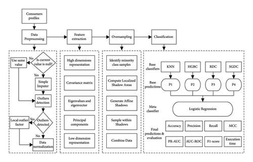
It discards majority class samples contain less information, and it ends up losing information. Moreover, the study in [13] uses ConvLSTM for classification of theft and honest samples by reshaping the energy usage into a 2-D matrix. This study achieves better results; however, it increases computational costs. Electricity consumption data contain redundant information and irrelevant features, which increases computational overhead and reduces the generalization of the final classifier. Study in [35] explains that DL models are suffered from high computation while processing redundant information.We proposed a stacked ensemble method to address the above issues in electricity theft. The process of the proposed method can be observed in Figure 2 and section Theft Detection Framework.
3. Theft Detection Framework
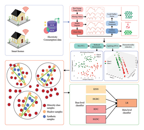
In this research, the suggested system model works in four steps and can be observed in Figure 3. The missing values and outlier detection are performed in the first unit. The curse of high dimensionality and class distribution issues are addressed in the second and third units, respectively. In the last unit, the cleaned data are fed to the stacked ensemble network. This network classifies energy consumption samples at a base level, where four strong machine learning classifiers are integrated. These classified samples are then fed to the meta level of this network, where a single classifier is used for second-stage classification. Finally, we perform a comparative analysis of the suggested framework using ADASYN and ICA for data augmentation and dimensionality reduction, respectively. Furthermore, a complete flowchart can be seen in Figure 2.
4. Data Preparation
This section of research represents the preprocessing of the dataset along with missing values imputation and outlier treatment. Furthermore, feature engineering is performed on electricity consumption data. Lastly, the class imbalance issue is further discussed.
4.1. Data Description
The energy consumption dataset is obtained from smart meters and publicly released by SGCC. The dataset consists of the daily energy consumption of 10000 consumers from January 01, 2014, to October 31, 2014, and is characterized as a time series. The samples are categorized between two classes’ theft and honesty, where 9100 samples belong to the normal class, and the rest of the 900 samples relate to the theft class. Furthermore, detail about the dataset can be observed in Table 2 [36].
| Time frame | Normal consumers | Theft consumers | Total consumers |
|---|---|---|---|
| Jan-01-2014 to Oct-31-2014 | 9100 | 900 | 10000 |
4.2. Retrieving Missing Values
4.3. Outlier Treatment
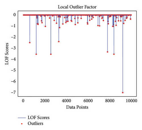
Realistic energy consumption data contain some missing values known as outliers that have a negative impact on the training of the classifier. This increases the training time and affects the performance of the classifier. The local outlier factor (LOF) presented in [38] is used to mitigate the outliers in a dataset and recover the data. Figure 4 exhibits the LOF score and outliers in the dataset.
4.4. Data Scaling
5. Addressing Class Distribution
5.1. Localized Random Affine Shadow Sampling
The class imbalance issue is one of the major concerns in the electricity dataset. As normal (honest) samples are easily available, theft samples are rarely available in the historical data. This huge class difference causes the theft detection framework to have misleading results toward the majority class while neglecting the minority class. Working with electricity theft, the detection of theft samples is more important as compared to honest samples. It is a challenging task to establish a framework that precisely separates the minority class samples in imbalance learning, where there are many honest samples and few minority class samples. Therefore, we employed a new oversampling method that synthetically generates minority class samples to balance uniform class distribution. The LoRAS oversampling method developed by [39] is integrated in this research to balance between both classes. The minority class samples are dispersed throughout the feature space, which creates a hindrance for the theft detection framework to learn the features of the minority class that distinguish them from the majority class samples.
Initially, the LoRAS algorithm generates a set of shadow data samples from each of the data samples in the minority class. It generates shadow data samples by adding noise to the original minority class sample. A function often known as sample variance of the feature decides how much noise is added in the sample.
-
Algorithm 1: Localized random affine shadow sample oversampling.
-
Initialize Algorithm
- (1)
Input: Training data
-
Output: Results
- (2)
Load dataset
- (3)
Training samples S = S1, S2,…, Sn⟹ S = Number of Samples
- (4)
Naff < k∗|Sp|
- (5)
For each minority class parent data p in Cmindo
-
where Cmin is minority class parent samples.
- (6)
Determine K-nearest neighbors for p and append p ⟶ neighbors
- (7)
Initialize neighborhood shadow samples as an empty list
-
For each parent data point q in neighborhood do
- (8)
Shadow points ⟵ draw |Sp| shadow samples for q drawing noise from normal distribution with corresponding standard deviation Lσ containing elements for each features Append shadow points to the neighborhood shadow sample.
-
Repeat
- (9)
Selected points ⟵ select Naff random shadow points form neighborhood samples affine weights ⟵ create and normalize random weights for selected points generate LoRAS sample point ⟵ selected points. Affine weights
- (10)
Append generated LoRAS sample points to LoRAS set
- (11)
UntilNgen resulting points are created003B
-
Return resulting set of generated LoRAS data points as LoRAS set
Theorem 1. It is stated that |F| > 2, and then, LoRAS algorithm has low variance as compared to SMOTE.
Proof. A shadow sample S is a random variable S = X + B that is synthetically generated by adding noise B to a minority data point X, which is named as Cmin, where noise B is added by following normal distribution N(0, σB).
The above equation is expressing that a LoRAS sample is generated by using random affine combination (RAC) of a set of shadow samples that are elements of neighborhood of X, which is denoted as NkX. The coefficients of the RAC are chosen randomly. The Dirichlet distribution (set of probabilities) is the coefficient of RAC a1…a |f|, in which all parameters assume that they have equal values to 1, which concludes that all features are equally important. For a random sample, i, j Σ1, …, |F|,
Here, covariance is a statistical measure that quantifies the correlation between two random variables, A and B, denoted as Cov (A, B). It represents how variations in one variable are associated with variations in the other variable.
6. Handling Curse of Dimensionality
6.1. Kernel Principal Component Analysis
Generally, there is a strong correlation between historical EC data, resulting in redundant features between input samples. The kernel principal component analysis (KPCA) [40] is an improved version of PCA, and it has the capability of extracting nonlinear relationship between features by incorporating nonlinear kernel function. PCA is a linear method that captures the most correlated features in the data. However, it faces trouble capturing intricate relationships and nonlinear patterns between samples in the data. KPCA discovers these nonlinear and complex features by mapping features using the kernel function. The KPCA technique computes principal components (PC) by leveraging the functionality of the kernel function. This helps KPCA to effectively discover hidden nonlinear and discriminative features that are unable to be detected by linear projection.
The detailed working of KPCA is found in Algorithm 2 [41].
-
Algorithm 2: Kernel principal component analysis.
-
Initialize Algorithm
- (1)
Input: Training data
-
Output: Results
- (2)
Load data construct the kernel matrix K
- (3)
Training samples S = S1, S2,…, Sn⟹ S = Number of Samples
- (4)
Ki,j = K(Xi, Xj)
- (5)
Step 2: Apply Matrix Gram K for kernel matrix . = K − 1n · K − K · 1n + 1n · K · 1n
- (6)
Step 3: apply Kak = λkNak to solve vector ai.
- (7)
Step 4: Compute kernel principal components yk (x) yk(x) = ϕ (x)Tvk = ∑Ni = 1akik(Xi, xj)
6.2. Adaptive Synthesis
-
Step 1: Determine the ratio between minority and majority samples by:
(12) -
where ma are the minority samples and mb are the majority samples. The algorithm is initialized when the value of d is lower than the threshold.
-
Step 2: Determine the number of synthetic data to be generated.
(13) -
where H is a total number of samples to generate. The β is the desirable minority to majority data ratio after ADASYN.
-
Step 3: Determine the nearest neighbors for minority samples and find the value of ri.
(14) -
where ri shows the influence of the majority class for every nearest neighbor.
-
Step 4: Determine the number of synthetic samples required to generate per nearest neighbor.
(15) -
Step 5: Choose two minority samples xi and xzi in the selected nearest neighbor randomly. Then, calculate the new synthetic sample.
(16) -
where λ is a random value between 0 and 1. Si is a synthetic sample. The xi and xzi are the minority samples in nearest neighbor. Algorithm 3 represents the detailed working of ADASYN oversampling method [42].
-
Algorithm 3: Adaptive synthesis.
-
Initialize Algorithm
- (1)
Input: Training data
-
Output: Results
- (2)
Load data set
- (3)
Training samples S = S1, S2,…, Sn⟹ S = Number of Samples
- (4)
Step 1: Calculate the ratio between majority and minority samples d = ma/mb (1) ma and mb minority and majority class samples, respectively.
- (5)
Synthetic samples generated for minority class. H = (mb − ma) × β (2) β denotes synthetic required samples and its range is (0, 1)
- (6)
Calculate Euclidean distance for each minority class sample by using K-nearest neighbor algorithm and also the ratio is calculated. Rx = δx × K−1, x = 1, …, ma (3) δx is majority class samples from K-nearest neighbor RnX = (4)
- (7)
Number of synthetic samples from each minority sample is calculated by gx = Rnx × S (5). For every synthetic gx, data are generated, by equation (6) Hx = ux + (uzx − ux) × λ (6), where (uzx − ux) is the difference in vector n dimensions and λ is a random number.
7. Feature Engineering
7.1. Independent Component Analysis (ICA)
ICA [43] is an unsupervised ML approach, and we employed it to tackle high-dimensional data. This method initiates by identifying fundamental trends within the dataset, which could manifest as thematic categories like sports or politics in textual data, or predominant trends in time-series data. For feature reduction, ICA serves as an effective alternative to PCA. ICA involves a linear decomposition of observed data into statistically independent components (ICs). The model posits x = As, where x represents the observed signal vector, A is a scalar matrix denoting the mixing coefficients, and s is the vector of source signals. ICA determines a separating matrix W such that y = Wx = WAs, with y being the vector of ICs. Independence stands as a more robust assumption than decorrelation achievable through techniques like PCA or factor analysis. In ICA, independence is conceptualized as each component offering no insight into the higher-order statistics of other components. Despite this, various methods exist for estimating ICA, and the algorithm for ICA can be found in Algorithm 4 [43].
-
Algorithm 4: Independent component analysis.
-
Initialize Algorithm
- (1)
Input: Training data
-
Output: Results
-
Step 1 Preparing data
- (2)
Load dataset
- (3)
Training samples S = S1, S2,…, Sn with number of x features x = S = Number of Samples
- (4)
Normalize each feature fi by (fi − mi)/2σi, where miandσi are the mean and standard deviation of fi, respectively.
-
Step 2 Performing ICA
- (5)
Apply ICA to the new dataset, and store the resulting weight matrix W of dimension (N + 1) × (N + 1).
-
Step 3 Shrinking small weights
- (6)
For each N + 1 independent row vector Wi of W, compute the absolute mean ai = .
- (7)
For all wij in W, if |wij| < α . ai, then shrink |wij| to zero, where α is a small positive number.
-
Step 4 Extracting feature candidates
- (8)
For each weight vector Wi, project it onto the original input feature space, i.e., delete weights wic = (wi, N + 1) corresponding to the output class, resulting in new weight matrix W of dimension (N + 1) × N to the original input data x, construct a (N + 1)-dimensional vector whose components are new feature candidates.
-
Step 5 Removing unappropriate features
- (9)
From features F = fi = Wix, i∑1 … N + 1. Then set Fs = F
- (10)
For each feature fi, if corresponding weights for class wic is zero, then exclude fi from Fs.
- (11)
For each feature fi, if corresponding weights wij = 0 for all j ∑1,…,N, then exclude fi from Fs.
- (12)
Resulting Fs contain final N extracted features.
7.2. Stacked Ensemble Architecture
Stacked ensemble method first suggested by [44]. The primary goal of stacked ensemble method is to reduce generalization errors in ML models. As explained in [36], the stacked ensemble method is the advanced form of cross-validation. It integrates multiple groups of learners using the winner-takes-all approach to boost overall prediction efficiency.
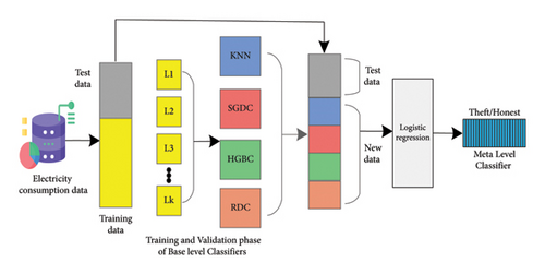
In the stacked ensemble method, multiple groups of learners are sorted in a hierarchical structure at a base level, where predictions are made on the data. The predictions from base learners serve as the input for the meta level. The stacked ensemble method consists of three major components. First, the training data are sliced into k nonintersecting subsets for training the classifiers. Second, a group of multiple learners is selected for the base level to make predictions on the validation set. Finally, the predictions from base learners serve as input features for second-stage classification at the meta level. The meta-classifier is trained on predictions from the base classifier as the target variable. Afterward, unseen data are passed to the trained meta-classifier for final predictions. In the first layer (K-fold), the preprocessed, clean, and balanced dataset X is split into a training dataset Sn and a test dataset Tq.
The training dataset Sn = Xn, yn, n = 1, 2, …, N is further split into K-folds (F1, F2, …, Fk), where X are features and y is the target variable. The test dataset Tq = (Xq), q = 1, 2, …, Q. On the second component, referred as base-level layer, it involves of P base models (Mp), defined as M1, M2, …, Mp. For every base learner (M1, M2,…, MP), distinct trainings are performed with K trainings and 1/k samples are set aside for the testing process to make predictions. The predictions form all base learners are combined with their actual labels and create new data. These new data are then fed to the meta-level classifier (Ymeta) as (y1, y2, …, Yp) for training and final predictions. The integrated stacked ensemble architecture can be observed in Figure 5. The methodology of the stacked ensemble framework can be observed in Algorithm 5.
-
Algorithm 5: Ensemble stacking.
-
Input: Training dataset D = (X1, Y1), (X2, Y2), …, (Xn, Yn); Base-Level Classifier L1, L2, …, Ln; Meta-Level Classifiers J.
- (1)
for t = 1,2, …, T do
- (2)
ht = Lt (D);
- (3)
end for
- (4)
D’ = ϕ
- (5)
for i = 1, 2, …, m do
- (6)
for t = 1, 2, …, T do
- (7)
zit = ht (xi);
- (8)
end for
- (9)
D′ = D′ U ((zi1, zi2, …., ziT), yi);
- (10)
end for
- (11)
h′ = L (D′)
-
Output: H(x) = h′ (h1(x), h2(x), …, hT(x))
7.3. K-Nearest Neighbor
-
Step 1: Select the training and testing samples. There are n number of groups for training and testing samples. Each group has x number of features and labels ai.
-
Step 2: Calculate the Euclidean distance d for number of groups in training and testing samples. Euclidean (E) = (1)
-
Step 3: The labels and corresponding distance used to create a new samples collection of the data samples.
(17) -
Step 4: Arrange the calculated distance A and labels ai according to Euclidean distance (E).
-
Step 5: Choose the samples from the arranged calculated distance A.
-
Step 6: Select the class of label according to the highest frequency as the final result for testing data.
7.4. Stochastic Gradient Decent Classifier (SGDC)
- (1)
Compute the derivative of the loss function for each feature; , where x is the features, yhat represents predicted labels, and y is the actual value.
- (2)
Find the gradient of the loss function in step 1 with respect to each feature in the dataset. This shows the direction of the minimum increase of the loss function and the direction toward a minimum of the function.
- (3)
Select a random initial feature value from the dataset to start theta0.
- (4)
Update the feature value for each iteration in the direction of the negative gradient. This updates the feature values in the direction where the loss function is decreased.
- (5)
Calculate the step size using: Step size = Gradient ∗ learning rate. This determines the update size, which will be used for feature values in each iteration.
- (6)
Find new feature value by following the formula: New value = old value–step size. New feature value is calculated by subtraction step size () from previous feature value. This step is continued for each feature. We subtract the step size because the new value is updated perpendicular to the gradient.
-
Algorithm 6: Stochastic gradient decent classifier.
-
Initialize Algorithm
- (1)
Input: Training data
-
Output: Results
- (2)
Load dataset
- (3)
Training samples S = S1, S2,…, Sn ⟹ S = Number of Samples
- (4)
Determine the derivative of loss function for each feature J(0) = , where y is the actual value and is predicted value in term of X.
- (5)
Calculate the gradient of loss function.
- (6)
Select a random initial value for the feature to start θ
- (7)
Update the gradient function by inducing the feature value
- (8)
Calculate step size by (Step size = Gradient ∗ learning Rate)
- (9)
Compute new feature value (New value = old value − step size)
- (10)
New value in opposite direction of the gradient. θ1 = θ0(stepsize∗j(θ))
- (11)
Shuffle the data points after each iteration
- (12)
Repeat 5 to 8 unless the gradient becomes closer to zero.
7.5. Ridge Classifier
It modifies the logistic regression (LR) cost function by including an L2 regularization penalty, which prevents the model from overfitting. Ridge classifier consists of three working phases explained below.
7.5.1. Initial Phase
- (1)
Alpha: It is used to improve classification and to overcome the variation of estimations. It is known as regularization constant.
- (2)
Max iteration: Defining how many iterations are used for solvers.
- (3)
Solver: There are many internal solvers in the ridge classifier training samples. For some instances, the auto option chooses an appropriate solver (i.e., Cholesky kernel, sparse cg, and Cholesky).
7.5.2. Fit Phase
A matrix X and a vector Y are provided to the classifier during fit phase. The feature vector that maps to the class y that is in the corresponding element in the vector Y corresponds to each row x of the matrix X, while the classifier creates a coefficient vector that best fits all of the data after learning from the data.
7.5.3. Prediction Phase
In this part, the classifier generates the classes for every row of the matrix by incorporating the matrix X and vector Y. Moreover, the working of the ridge classifier can be observed in Algorithm 7 [47].
-
Algorithm 7: Ridge classifier.
-
Initialize Algorithm
- (1)
Input: Training data
-
Output: Results
- (2)
Load dataset
- (3)
Training samples S = S1, S2,…, Sn ⟹ S = Number of Samples
- (4)
Step 1: For each test data X ϵ X-test.
- (5)
Calculate the classification parameter vector = , where λ is the regularization parameter and i represent each class.
- (6)
Step 2: Perform projection of new test samples x onto the subspace of each class i by as
- (7)
Calculate distance between the test space sample x and the class specific subspace xi
- (8)
The test sample x is assigned to that class whose distance is minimum.
7.6. Histogram Gradient Boosting
Histogram Gradient Boosting (HGB) classifier is an advanced version of gradient boosting technique [48]. The traditional gradient boosting is a greedy algorithm, which considers all possible decision tree splits and selects the optimal split. This approach increases the computation time when working with large datasets. However, the HGB method converts feature values into bins or histograms. Each histogram represents a specific range of feature values, which helps the algorithm to calculate the sum of gradients for each histogram. This helps the algorithm in faster processing speed and reduces memory usage as compared to traditional gradient.
The training sample S possesses a number of n features in the dataset. The histogram of equal density is created for each feature, and all feature values are replaced by the index of histograms. While computing the gain, the left child, right child, and current node have the necessary sum of gradients. The computation process is more faster by adding the gradients stored in every bin. Initially, GB has the complexity of O(n log n) and is changed to O (nbinss) after applying histograms. In gradient boosting algorithm, the value of bins can be changed by maxbin parameter. In short, this is the main reason for increasing the performance of the modified GB framework. Furthermore, working of HGB is explained in Algorithm 8 [49]
-
Algorithm 8: Histogram gradient boosting.
-
Initialize Algorithm
- (1)
Input: Training data
-
Output: Results
- (2)
Load dataset
- (3)
Training samples S = S1, S2,…, Sn⟹ S = Number of Samples
- (4)
Node Set ⟵ 0 ⟹ tree nodes in current level
- (5)
Row Set 0, 1, 2,…⟹ data indicate in tree nodes
- (6)
for i to d do
- (7)
for node in node Set do
- (8)
used Rows ⟵ row se [node]
-
for k = 1 to m do
-
H ⟵ new Histogram ()
-
⟹ Build histogram
-
for j in used rows do
-
bin ⟵ I.F[k][j].
-
bin H[bin].y ⟵ H[bin].y + I.y [j]
-
H[bin].n ⟵ H[bin].n + 1
- (9)
Find the best split on histogram H.
- (10)
Update rowset and nodeSet according to the best split points.
7.7. Logistic Regression
-
Algorithm 9: Logistic regression algorithm.
-
Initialize Algorithm
- (1)
Input: Training data
-
Output: Results
- (2)
Load dataset
- (3)
Training samples S = S1, S2,…, Sn ⟹ S = Number of Samples
- (4)
Create matrix of input features Z
- (5)
Multiply Z matrix with weights matrix
- (6)
Pass the data to Sigmoid Function (Y) g(z) = 1/1 + e−x
- (7)
Map the data on S curve
- (8)
Samples are classified by threshold with S curve
8. Simulation Results and Discussion
8.1. Performance Metrics
For the evaluation of our proposed scheme, comprehensive performance metrics were used on the test data (30%) to assess the robustness and effectiveness of the suggested scheme for malicious sample identification.
8.1.1. Confusion Matrix
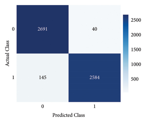
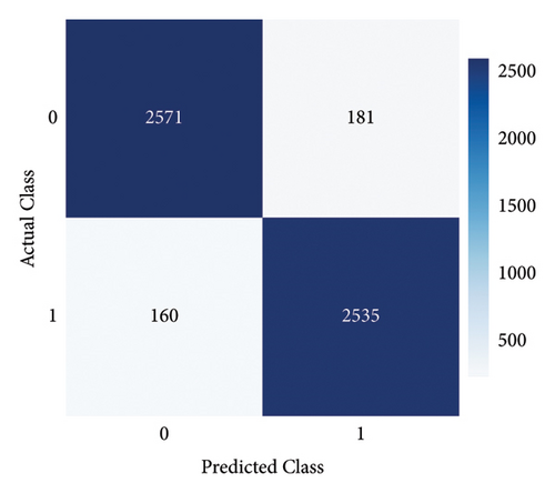
The CM is a method used to summarize the possible distinct outcomes of the classifiers and can be observed in Figure 5. The CM is based on true positive (TP), false positive (FP), true negative (TN), and false negative (FN). TP (1, 1) shows the theft consumers accurately detected as theft by the model. FP (0, 1) displays honest consumers identified as theft by the model. TN (0, 0) shows the normal consumer identified as normal by the mode. FN (1, 0) shows the theft consumer identified as normal by the classifier. Based on these performance metrics, we evaluated our proposed scheme by incorporating different metrics, such as accuracy, precision, recall, and F1 score.
8.1.2. Accuracy
8.1.3. Precision/Positive Prediction Score (PPS)
8.1.4. Recall/True-Positive Rate (TPR)
8.1.5. F1 Score
8.1.6. Matthew’s Correlation Coefficient (MCC)
The MCC is used to measure the performance of binary classifier, and it is a single value, which ranges from +1 to −1. The classifier with a value closer to +1 indicates the best performance, where as the value negative to −1 refers to the worst performance. It is defined as: .
8.1.7. AUC Score
It is the most reliable metrics while working with imbalanced dataset. It shows the overall performance of the classifier, the higher value indicates the best performance of the classifier.
8.1.8. Area under the Receiver Operator Curve (AUC-ROC)
The classifier with higher AUC-ROC perfectly separates both classes. The AUC-ROC plots TP against FP on the y-axis and x-axis, respectively. It ranges from 0 to 1 when a classifier falls below 0.5, which shows that the classifier is randomly guessing.
8.1.9. Area under Precision-Recall Curve (PR-AUC)
While working with the electricity consumption dataset, the PR-AUC is the most appropriate evaluation metric, which focuses on minority class (theft) or class of interest. PR-Curve is the graphical representation of precision and recall while working on a dataset with unequal class distribution. It is obtained by the average of precision calculated at each recall threshold, which makes it useful diagnostic for the detection of class of interest.
8.1.10. Execution Time
It is the time taken by the model to process the information passed to the input. It is measured in seconds, nanoseconds, and microseconds.
8.2. Simulation Settings
The experimental setup is performed on Intel Core i5 processor with 16 GB RAM as illustrated in Figure 3. The proposed framework is implemented and tested using Python IDE. The daily electricity consumption data are taken from SGCC [36], where 9100 samples are benign, and the rest of 900 samples are suspicious and makes the proportion of 91% of honest samples, and 9% are theft samples as explained in Table 2. We take the best experimental values of our proposed method after many simulations.
8.3. Experimental Results and Discussion
In this section, we evaluated our proposed framework, by accuracy, precision, recall, AUC score, AUC-ROC, and F1 score.
8.4. Discussion of Simulation Results with LoRAS and KPCA
In this case study, we employed the LoRAS algorithm to mitigate the class distribution issue and KPCA for feature engineering on the dataset as delineated in Table 3. The proposed scheme combination offers high accuracy as LoRAS generates more realistic samples by integrating localized random affine on the minority class for sample augmentation. The majority class samples predominate over the minority class samples, resulting in the bias of the classifier toward the majority class. Furthermore, the integration of KPCA helps to reduce computational time by discarding the redundant information from the dataset.
| Classifiers | Accuracy | AUC score | F1 score | Precision | Recall | MCC | AUC-ROC | PR-AUC | Execution time (s) |
|---|---|---|---|---|---|---|---|---|---|
| KNN | 65 | 65 | 50 | 87 | 35 | 37 | 65 | 77 | 3 |
| HGBC | 96 | 94 | 93 | 96 | 94 | 91 | 94 | 97 | 48 |
| RDC | 66 | 94 | 74 | 60 | 96 | 40 | 65 | 79 | 1 |
| SGDC | 60 | 60 | 72 | 56 | 76 | 33 | 63 | 78 | 1 |
| Proposed | 97 | 97 | 97 | 98 | 95 | 93 | 97 | 98 | 1 min 7 |
| GridSearch | 97.5 | 97 | 97 | 99 | 95 | 93.51 | 97 | 98 | 2 min 27 |
| CNN | 93 | 92 | 94 | 93.5 | 93 | 88 | — | — | 5 min 38 |
| LSTM | 55 | 58 | 48 | 65 | 56 | 18 | — | — | 8 min 53 |
Figure 6 illustrates that the proposed scheme attains superior performance, showcasing higher values. Notably, the HGBC classifier stands out with commendable results, benefiting from its affiliation with the boosting family.
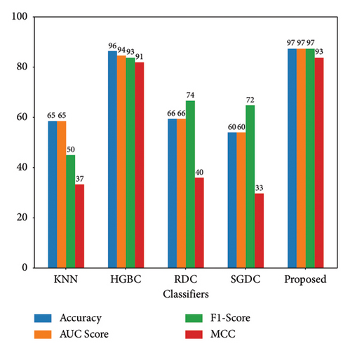
It can be clearly observed in Figure 6 that the suggested method achieves superior values. Notably, the HGBC classifier archives remarkable results as compared to other base classifiers due to the affiliation of HGBC with the boosting family. However, our proposed method surpasses the HGBC by achieving 97% accuracy and 93% MCC as compared to HGBC with 96% accuracy and 91% MCC. The complexity of HGBC makes less efficient than our proposed model. HGBC lacks due to the complexity of the algorithm.
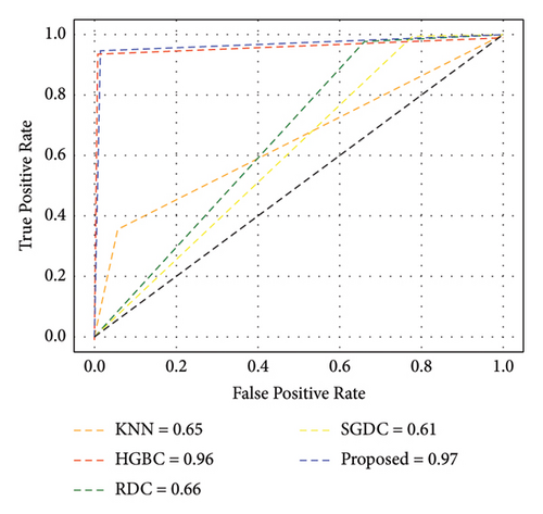
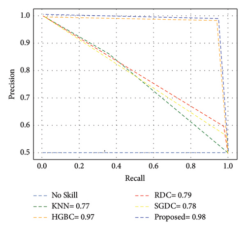
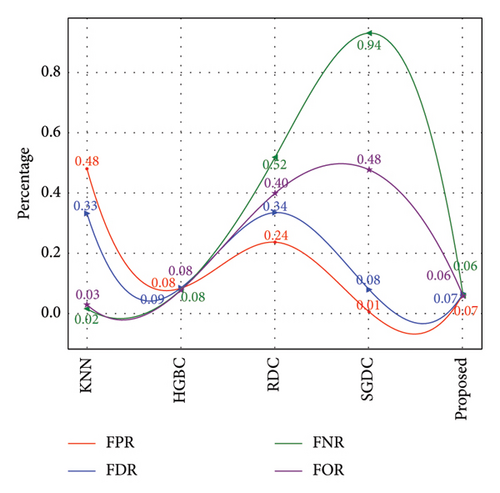
Furthermore, Figure 7 exhibits that our proposed model achieved the highest AUC-ROC score of 97%, which is the highest value among all other benchmark techniques. Figure 8 illustrates the PR-AUC of our proposed model, and it is proved that the proposed scheme surpasses all other techniques by achieving 98% of PR-AUC. Moreover, we evaluated our proposed model by using CM. As seen in Figure 9, the proposed approach achieved the lowest FN. As delineated in Table 3, our proposed approach achieved 93% MCC score, which is higher than all other techniques. However, SGDC achieves the lowest MCC values as it is stuck in capturing the complex patterns in the data that cause lower MCC. To further verify the effectiveness of our proposed method, we also calculated the values of FPR, FOR, FNR, and FDR in Figure 10 for base and meta-level classifiers. The values near the zero clearly indicate the effectiveness of our proposed method.
8.5. Discussion of Simulation Results with ADASYN and ICA
The simulation values are quite different as we apply ICA for feature engineering and ADASYN for oversampling the minority class in this case study. We can see the bar plot in Figure 11, and our proposed method outperforms other techniques with the combination of ICA and ADASYN. However, simulation values are lower than a previous case study.
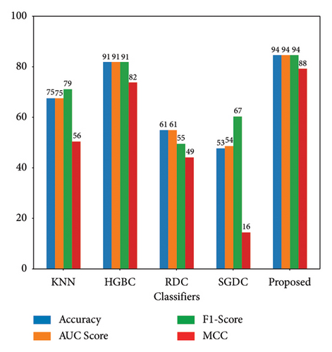
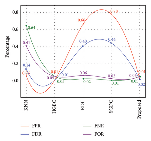
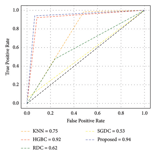
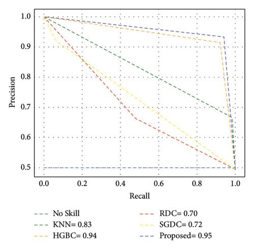
Since ICA is a linear method, it might not be appropriate for handling nonlinear datasets. This limitation results in longer processing time for the classifiers. Moreover, ADASYN is sensitive to noise, which cases lower performance of this combination. Figure 12 illustrates that the proposed method achieves an AUC-ROC score of 94%, which is lesser than the previous one with 97%. Similarly, Figure 13 exhibits the overall PR-AUC curve with 95%, which is quite lower than the previous case study with 98%. To validate the effectiveness of the previous case study, CM can be observed in Figure 14. Here, FN needs to be reduced because in electricity theft, these are the real culprits that steal electricity and affect the stability of the smart grid. Moreover, the results in Table 4 exhibit the numerical values of the proposed method with ICA and ADASYN. Finally, Figure 15 clearly proves the superiority of the previous study as the FOR, FNR, FDR, and FPR values are a little bit higher.
| Classifiers | Accuracy | AUC score | F1 score | Precision | Recall | MCC | AUC-ROC | PR-AUC | Execution time (s) |
|---|---|---|---|---|---|---|---|---|---|
| KNN | 75 | 75 | 79 | 66 | 97 | 56 | 75 | 83 | 2 |
| HGBC | 91 | 91 | 91 | 90 | 92 | 82 | 91 | 93 | 17 |
| RDC | 61 | 61 | 55 | 65 | 47 | 49 | 61 | 69 | 1 |
| SGDC | 53 | 54 | 67 | 51 | 98 | 16 | 54 | 75 | 1 |
| Proposed | 94 | 94 | 94 | 93 | 95 | 88 | 94 | 95 | 1 min 13 |
- Bold refers to higher values.
9. Conclusion
In this study, we analyzed the limitations of existing theft detection methods in smart grids. As the smart grid is the heart of a smart city, any disturbance in smart grid operation will paralyze all the functionality of the smart grid. We proposed a stacked ensemble method for detecting electricity theft in a smart grid. Furthermore, the effectiveness of the proposed method was tested with two different case studies. In the first study, we combine LoRAS and KPCA for data augmentation and feature engineering. Meanwhile, in the second study, we use ADASYN and ICA for oversampling and dimensionality reduction. Finally, all simulation results verify the effectiveness of the first case study.
10. Future Work
We have developed a stacked machine learning-based model for the mitigation of electricity theft in smart grids to enhance the functions of smart cities. In future developments, the mitigation of nontechnical losses moves toward deep learning methods. Deep learning presents a viable alternative to traditional machine learning models, which could find it difficult to handle the processing demands of large datasets. Deep learning algorithms can analyze large amounts of data quickly and accurately by utilizing complex neural network designs. This makes it possible to identify possible cases of electricity theft more precisely and promptly.
Conflicts of Interest
The authors declare that they have no conflicts of interest.
Authors’ Contributions
Muhammad Hashim (M.H.), Laiq Khan (L.K.), and Nadeem Javaid (N.J.) conceptualized the study. L.K., N.J., and Ifra Shaheen (I.S.) performed the data curation. M.H., L.K., Zahid Ullah (Z.U.), and I.S. carried out formal analysis. L.K., N.J., and Z.U. assumed investigation responsibilities. M.H. and L.K. devised the methodology. L.K. and Z.U. overseen the project administration. M.H. and Z.U. provided the resources. M.H. managed software resources. L.K. and N.J. supervised the study. M.H., L.K., and N.J. conducted validation procedures. M.H., L.K., and Z.U. conducted the data visualization. M.H., L.K., N.J., Z.U., and I.S. wrote the original draft of the manuscript. M. H., L.K., and Z.U. reviewed and edited the manuscript. Every contributor has thoroughly examined and endorsed the finalized manuscript for publication.
Acknowledgments
The authors would like to thank the CRUI for the support of APC under the CARE-CRUI Agreement with Wiley.
Open Research
Data Availability
The data used to support the findings of this study are available from the corresponding author upon request.


