Accurately forecasting electricity demand is crucial for maintaining the balance between supply and demand of electric energy in real-time, ensuring the reliability and cost-efficiency of power system operations. The integration of numerous active loads and distributed renewable energy sources into the grid has led to increased load variability, rendering the traditional point forecasting approach inadequate for meeting the evolving needs of the power system. Probabilistic forecasting, which predicts the complete probability distribution of loads and provides more extensive information on load uncertainty, has emerged as a key solution to address these challenges. The long short-term memory (LSTM) model, known for its strong performance in modeling long series, is commonly utilized in load forecasting. Therefore, this study focuses on short-term electric load probability forecasting for users in a specific park in Yantai. We propose a short-term load probability forecasting model based on integrated feature selection (IFS), genetic algorithm (GA) optimization of LSTM, and quantile regression (QR), referred to as the IFS-GA-QRLSTM model. Initially, the integrated feature selection method is employed to identify the most influential factors affecting electric load, optimizing the model’s input features and reducing data redundancy. To address the subjective nature of parameter selection in the LSTM model, we use a GA to optimize model parameters. The combination of optimized LSTM with QR enables direct generation of quantile load predictions, which are further used in kernel density estimation to construct the probability density distribution. We compare the proposed method with five basic models, QRLSTM, IFS-QRCNN, IFS-QRRNN, IFS-QRLSTM, and IFS-QRGRU, for point prediction, interval prediction, and probability prediction. Experimental results demonstrate that the proposed method in this paper exhibits better prediction performance, smaller prediction errors, and greater effectiveness compared to the aforementioned models.

1. Introduction

1.1. Background of the Study

The power system plays a crucial role in ensuring the normal functioning of the national economy and the daily lives of residents. To maintain the stability and reliability of the power system, accurate predictions of future power loads are essential to balance power generation with demand. In recent years, with an increasing focus on low-carbon environmental protection, new energy generation methods such as wind power, solar power, and hydroelectric power have emerged, among which the research on photovoltaic power generation hours prediction has achieved better results [1]. Although these sources are clean, their generation is susceptible to weather conditions and temperature, leading to complex and fluctuating load data. Consequently, predicting power loads in this new type of power system has become a key research area for scholars globally.

Before the power system became as complex as it is today, forecasting power loads only required providing a single point forecast to meet grid requirements [2]. However, with the introduction of new energy generation methods, the uncertainty in the power system has increased significantly. There is now a pressing need for a more precise method to assess this uncertainty. Probabilistic load forecasting emerges as a viable solution to this challenge [3]. This approach can offer a prediction interval [4] and the corresponding probability density function of the predicted load value at a specified confidence level. By doing so, it allows for a more accurate measurement of the uncertainty in load prediction and the distribution of predicted load values. This capability is crucial for power generation systems to make informed risk decisions and optimize power dispatching.

While probabilistic forecasting can assess the uncertainty of load forecasting, achieving high forecasting accuracy still relies on robust data support. The datasets used in the current literature are mostly public, which can allow scholars to reproduce their research results, but lack timeliness and are less convincing. At the same time, the existing research does not pay enough attention to the selection of important data features and tends to focus more on the research of new algorithms, overlooking the importance of data itself to the model. To address this gap, we propose a novel feature selection method to identify the variables most relevant to the target variables for input into the model. This paper not only focuses on point forecasting but also introduces interval forecasting and probabilistic forecasting of loads to offer more valuable insights for future load forecasting. For model selection, we leverage deep learning, a widely used approach, and further enhance prediction accuracy by optimizing model parameters through an optimization algorithm. This approach aims to effectively tackle the challenges in load forecasting.

1.2. Literature Reviews

The current research on power load forecasting can be broadly classified into four categories: ultra-short-term, short-term, medium-term, and long-term load forecasting. Ultra-short-term load forecasting involves predicting future loads at a granularity below the hourly level, typically used for real-time scheduling and control [5, 6]. Short-term load forecasting, on the other hand, focuses on forecasting loads from a few hours to a few days ahead, primarily for daily or weekly power generation planning [7, 8, 9, 10]. Medium-term and long-term load forecasting operate on monthly and yearly time scales, respectively, and are primarily utilized for power grid maintenance, reconstruction, and planning [11, 12]. However, due to the significant time gap between medium-term and long-term forecasting, the resulting prediction errors can be substantial, limiting practical applications [13, 14, 15]. Ultra-short-term forecasting tasks are usually managed by the power grid and dispatching departments due to their high real-time demands. As a result, the majority of research efforts in this area are concentrated on short-term power load prediction.

The single-point methods for short-term power load forecasting can be broadly classified into two types: traditional forecasting methods and modern forecasting methods. Traditional methods include time series forecasting [16], Kalman filter [17], exponential smoothing model [18], and multiple linear regression [19]. These methods model historical loads to predict future loads but are limited by their simple structure and linear relationship fitting capability, resulting in lower prediction accuracy, especially when dealing with nonlinear data. In contrast, modern methods such as machine learning [20] and deep learning [21] have gained popularity in the big data era. These methods are adept at handling fluctuating data and improving nonlinear fitting capabilities, leading to higher prediction accuracy in power forecasting. In this context, Aslam et al. [22] compared the performance of different artificial neural networks and machine learning methods in forecasting electricity generation in residential and commercial sectors and found that the efficiency of these forecasting methods highly depends on historical data, which fully demonstrates that data preprocessing is a key factor affecting model performance. Giacomazzi et al. [23] explored the ability of the transformer architecture in short-term hourly load forecasting for the present and different power grid levels. The results showed that its forecasting performance is far inferior to the long short-term memory (LSTM) model. However, when the transformer applied at the substation level with a subsequent aggregation to the upper grid-level, it appears to offer remarkable improvements over the LSTM approach. To better assist researchers in making meaningful model choices, Hopf et al. [24] reviewed 421 forecasting models from 59 past studies and found that LSTM and the combination of neural networks with other methods can improve the accuracy of forecasting results.

In view of the current new power system, domestic and foreign scholars have conducted research on how to measure the uncertainty of power load. Haben et al. [25] reviewed some research on low-voltage forecasting, and they pointed out that the challenges faced by current smart meter forecasting are similar to those of low-voltage forecasting, both of which have instability and require probabilistic forecasting to estimate their associated uncertainties. In the 2014 Global Energy Forecasting Competition, Xie and Hong [26] proposed a probabilistic load forecasting solution for measuring load uncertainty, and since then, probabilistic forecasting of loads has become a hot topic in academic research. Xu et al. [27] proposed a probabilistic load prediction method for individual buildings and established an ANN model for probabilistic normal load prediction and a statistical model for probabilistic anomalous peak prediction. Wang et al. [28] used the constrained quantile regression averaging method (CQRA) for the integration of multiple single probabilistic prediction models and demonstrated that the predictive performance of the integrated prediction was significantly improved compared to the single prediction. Dengwu et al. [29] proposed a power load interval prediction method combining deep learning and quantile, which can output the prediction results of multiple quantiles and then obtain the load prediction interval at a given significance level. Literature [30] proposed a user-level short-term probabilistic load forecasting method for night economy. This method first used LightGBM for point forecasting, took the output obtained from point forecasting as the input of probability forecasting, then used kernel density estimation method to estimate the probability density and forecast interval of future short-term load of different night economy users, and conducted experiments on multiple types of night economy users. All of them showed good effect. Literature [31] proposed a probabilistic load prediction method for individual users by replacing the mean square error with the pinball loss as the loss function of the LSTM for model training, thus extending the traditional LSTM-based point prediction into a quantile form of probabilistic prediction. As feature variable selection is also one of the key factors affecting model training, Li Jinyang proposed to combine copula method and XGBoost algorithm, so as to select the most relevant influencing factors of power load. Then, this variable screening method was put into the three quantile prediction models of QRLSTM, QRF, and QRGB, and the experimental results showed that the prediction accuracy of the proposed models was improved [32]. Wei et al. [33] proposed a multifeature short-term power load forecasting method. First, the original load data were decomposed into N modes and one residual through variational mode decomposition VMD, and the N modal components were predicted by LSTM in a single variable. Then, the residual and weather and date features are combined together to make LSTM multifeature prediction. Finally, the above prediction results are taken as the whole feature to make multifeature load prediction through LightGBM. Experimental results show that the prediction error of this method is lower than that of traditional machine learning algorithms. In the literature [34], in order to alleviate the possible overfitting as well as high complexity problems of QLSTM models, it was simplified using nonconvex MCP regularization, and finally, the model parameters in LSTM and MCP were optimized by whale algorithm, which significantly improved the prediction accuracy of the model.

Based on the current research status, we introduce a novel IFS-GA-QRLSTM hybrid model for short-term load probabilistic forecasting. This model initially conducts feature screening by incorporating a feature selection algorithm to eliminate unnecessary features. Subsequently, the hyperparameters of the LSTM model are fine-tuned using a genetic algorithm and integrated with quantile regression to predict values at various quantile points. The results include point prediction, interval prediction, and probabilistic prediction of loads, demonstrating the enhanced performance of the proposed method in this study.

1.3. Contributions

Here are the main contributions of this article:

(1)
The dataset used in this study is from the real-time load data of users in a certain park in Yantai, which includes information on weather conditions, temperature, and wind direction. For the textual data, we have split and encoded it. At the same time, in order to comprehensively examine the feature factors that affect the load data, we have also extracted seven time-related factors that have a significant impact on it, ensuring the comprehensiveness of the features.
(2)
We propose a new integrated feature selection method, which is not limited to the feature selection of a single model but integrates RF, XGBoost, and LightGBM models and combines the feature importance scores obtained by their respective training through a weighted method, so as to obtain the final feature importance scores. Finally, it filters the features based on a predefined score threshold to select the most important features.
(3)
We propose to optimize the hyperparameters of LSTM by genetic algorithm, which includes the number of LSTM layers, dense layers, hidden layer neurons, and dense layer neurons, in order to further improve the prediction accuracy of the model.
(4)
In this study, an LSTM model optimized using genetic algorithms is integrated with a nonlinear quantile regression model to provide probabilistic load data predictions for a specific park in Yantai. The analysis of the prediction results is conducted based on three main aspects: point prediction, interval prediction, and probability prediction.

2. Methodologies

2.1. Integrated Feature Selection

Feature selection is a key part of multifeature data processing, which cannot only reduce the complexity of data but also significantly improve the prediction accuracy of the models. The feature selection method of a single model is introduced above. Although this method is widely used by scholars, numerous research clearly show that the feature importance rankings given by different models vary significantly. This variability undermines the robustness of feature selection results from a single model. It is still necessary to find a new feature selection method to further solve the above problems. Based on the above problems, we propose a new feature selection method based on an integrated idea of machine learning, which is no longer limited to feature selection of a single model but combines RF [35, 36], XGBoost [37, 38], and LightGBM [39, 40] models. The trained feature importance is weighted and fused in a certain way, and finally, the final feature importance ranking is given, and then the feature variables that meet the requirements are screened out according to the actual situation. Specific practices are as follows:

(1)
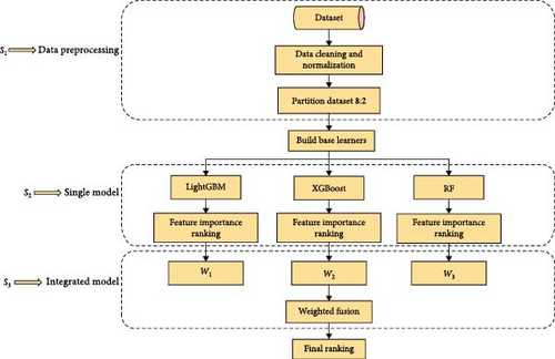
First of all, the data are preprocessed, including data cleaning and normalization operations.
(2)
The preprocessed data are divided into the training set and the test set according to the ratio of 8 : 2.
(3)
RF, XGBoost, and LightGBM models are established, respectively, and the above three models are taken as the base learners of the overall method. Then the segmented data are input into the above three models for training and testing.
(4)
Set the weighting coefficient w_i(i = 1, 2, 3) of each model, and according to the advanced degree of the above algorithms, order them from strong to weak as LightGBM, XGBoost, and RF, and set their coefficients as 0.5, 0.4, and 0.1, respectively, that is, w₁ = 0.5, w₂ = 0.4, w₂ = 0.4.
(5)
The feature importance scores of each feature obtained by the three base learners are denoted as , where j = (1, 2, …, n) represents the j feature and n represents the total number of features in the dataset.
(6)
Calculate the final feature importance score :

()

(7)
The importance scores of the above features are sorted in descending order, and the required number of features is selected according to the actual situation. The design process of the algorithm is shown in Figure 1.

Details are in the caption following the image — **Figure 1**
Open in figure viewer PowerPoint

Integrated feature selection design flow.

2.2. GA

The genetic algorithm was proposed by John Henry Holland in the 1970s as a global search method for solving various optimization problems [41, 42, 43]. It simulates the biological evolution process of natural selection and genetic mechanisms as described in Darwin’s theory of evolution. Through mathematical computation and computer simulation operations, it transforms the problem-solving process into a sequence resembling biological evolution, involving copying, crossover, and mutation of chromosome genes. This process screens a group of individuals to identify those best suited for the environment in order to obtain the optimal solution to the problem. The primary operations in a genetic algorithm are selection, crossover, and mutation, which collectively constitute the genetic operations. It can be represented as follows:

()

where C represents the coding mode of the individual, E represents the individual fitness function, P₀ represents the initial population, M represents the population number, ϕ represents the selection operator, Γ represents the crossover operator, ψ represents the mutation operator, and T represents the termination condition of the genetic algorithm.

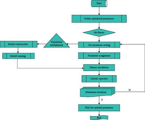
The implementation steps of genetic algorithm can be divided into five stages: chromosome coding, initial population, fitness evaluation, genetic operator, and termination condition judgment. The chromosome coding stage can be divided into two parts, namely, encoding and decoding. Encoding can be understood as a transformation method, that is, to convert the feasible solution of a practical problem into a representation suitable for genetic algorithms. Similarly, decoding is also a conversion method, that is, the conversion of genetic algorithm chromosomes to problem solutions. The operation of encoding and decoding is to facilitate the subsequent genetic algorithm operation. The initial population means that before establishing the algorithm model, the solution population in the search space needs to be defined in advance, and a series of parameters are set, including the maximum evolutionary algebra T, population size M, crossover probability P_c (generally set in the range of 0.4–0.99), and mutation probability P_m (generally set in the range of 0.001–0.1). Randomly generate M individuals as the initial group P₀. Next, it is crucial to establish the fitness function in the genetic algorithm, which serves as a metric for evaluating the relative quality of individuals within the population. In the approach outlined in this paper, the reciprocal of the mean square error (MSE) of the prediction model is utilized as the fitness value. After setting the fitness function, it is necessary to calculate the genetic operator, that is, select, cross, and mutation operations. Population P(t) underwent the above three genetic manipulations; the next generation of population P(t + 1) is obtained. The final step involves defining termination conditions to achieve the optimal solution for the problem. The algorithm terminates when the fitness function reaches a predetermined optimal value or when the maximum number of iterations is reached. The entire operational process of the algorithm is illustrated in Figure 2.

2.3. LSTM

LSTM, short for long short-term memory neural network, was introduced by Hochreiter and Schmidhuber in 1997 as a variation of the traditional RNN with significant changes in network structure. It addresses the issues of vanishing and exploding gradients present in RNN and greatly improves the modeling capabilities for long sequences [44, 45, 46]. Currently, LSTM is widely utilized in power prediction with stable performance. Its key components consist of the forget gate, input gate, cell state, and output gate. The typical unit structure and calculation formulas are as follows:

()

here W_f, W_i, W_c, and W₀, respectively, represent the weight of the forget gate, input gate, cell state, and output gate and b_f, b_i, b_c, and b₀, respectively, represents the offset item; σ represents the Sigmoid activation function; f_t represents the output of the forget gate;

, respectively, represent the updated output of the input gate and the new candidate value; C_t−1 represents the cell state at the previous moment; O_t determines the output part of the cell state; and h_t represents the final output. The gating mechanism of LSTM is illustrated in Figure 3.

2.4. Probabilistic Prediction Model

Quantile regression, a nonparametric statistical method, is extensively applied in forecasting [47]. This paper combines it with the LSTM algorithm, resulting in the QRLSTM model obtained by substituting the traditional LSTM model’s mean squared error loss function with the pinball loss. The model is trained by minimizing the pinball loss, and the expressions of its pinball loss function and minimization objective function are shown as follows:

()

where D is the sample quantity,

is the predicted value corresponding to quantile at time t, y_t is the actual observed value, PL_min is the objective function, and T is the total time interval.

When performing quantile regression based on the above objective function, there is one quantile corresponding to each model, and it is a common requirement to construct numerous prediction models in order to generate predicted values for multiple quantiles, a process that is time-consuming and labor-intensive. Furthermore, the prediction results can be unstable. To enhance the model further and enable it to simultaneously output predicted values for multiple quantiles, the pinball loss function can be adapted into the average pinball loss function. This modification allows for the direct derivation of prediction results for multiple quantiles. The expression of the average pinball loss function is as follows:

()

where APL_min is the minimum average pinball loss (i.e., the objective function), Q is all quantiles used, and |Q| is the absolute value of all quantiles.

Through quantile regression, we can obtain the predicted values of different quantiles corresponding to a certain time, but these predicted values are discrete points. To derive the probability density function of various predicted points, we must input the aforementioned series of quantile values into the kernel density estimation. This process will allow us to calculate the probability density function of the forecasted load. The specific steps are as follows:

Suppose that a series of predicted values obtained by quantile regression can be expressed as

, input them into the kernel density estimation as a set of sample data, and the resulting probability density function can be expressed as follows:

()

where f_e(y_t) denotes the estimated probability density function, h denotes the bandwidth, and K(⋅) denotes the kernel function, among which the more common kernel functions are uniform kernel function, triangular kernel function, gamma kernel function, Epanechnikov kernel function, etc. Since the Gaussian kernel function is mostly used in the probabilistic prediction study, this function is also selected for estimation in this paper, and its calculation formula is as follows:

()

where σ is the smoothing parameter of h, and by substituting Equation (14) into Equation (13), the final probability density expression estimated by Gaussian kernel function is obtained:

()

By using the above expression, the probability density function at any given point can be determined, enabling a better observation of the distribution of load data.

3. Data Preprocessing

3.1. Dataset Introduction

The dataset used in this paper is derived from the electricity load data of a park user in Yantai from January 1, 2018, 0:00:00, to August 31, 2021, 23:45:00, with a total of 128,157 pieces of data. It is collected every 15 min and contains five columns of meteorological characteristic data and one column of load data, including electricity load, weather conditions, maximum temperature, minimum temperature, daytime wind direction, and night wind direction. Among them, the weather condition, daytime wind direction, and night wind direction are text-based data. In order to explore the time correlation of the dataset selected in this paper, Figures 4, 5, 6, and 7, respectively, show the time series of load data in 1 day, 1 week, different months, and different years.

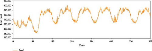
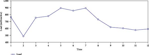
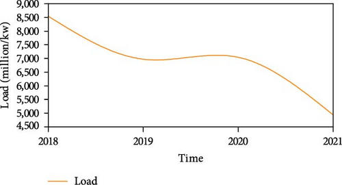
The figure clearly shows distinct peak and trough values in different periods of the day, suggesting that the number of days is also a factor impacting the load. The data show an obvious periodicity within a week, and its electricity consumption pattern is also very different in different months, and it also shows an obvious trend in different years. Therefore, based on the above analysis, we will extract time-related factors to ensure the integrity of load influencing factors.

3.2. Missing and Outlier Processing and Data Standardization

As for the missing value in the data, we use the method of filling to complete it. The specific method involves filling missing values by weighting the load value of the moment before and after the missing value, as well as the load values of the same moment from the previous and next day. Outliers and duplicate values in the data are minimal and are handled by direct elimination. To prevent errors from excessive data changes, the data in the dataset are normalized using the following equation:

()

The variables in the equation have the following meanings: Q^norm is the normalized value, Q is the value that needs to be normalized, and Q_max and Q_min are the maximum and minimum values before normalization, respectively.

3.3. Time-Dependent Feature Extraction and Coding

Based on the analysis of the time series diagram above depicting the power load of park users, it is evident that the power load is significantly influenced by time factors including days, week, months, and years. To comprehensively investigate the factors influencing load characteristics, additional meteorological factors need to be incorporated into the analysis. Then, seven time features related to the load, namely, year, month, day, weekday, weekend, week, and holiday, are extracted, and the extracted time-related features are combined with the above meteorological features and load data, and finally, compose a complete dataset. Then, for the text data in the dataset, it needs to be converted into numerical data for subsequent operations. The “Weather Conditions” feature column in the dataset looks like this: ”Multi-cloud/multi-cloud”, so the practice in this paper is to divide it into two columns according to “/”, start_weather before “/”, end_weather after “/”, and then encode the label. The encoding range is 0–16. Then, label coding is also carried out for the two text-type feature columns of daytime wind direction and night wind direction, and the encoding range is 0–27. Finally, a dataset containing one column of load data and 13 columns of feature data is obtained. The description and coding of characteristic variables in the dataset are shown in Tables 1 and 2.

Table 1. Characteristic variable introduction.

Input type	Variable name	Variable description
Target variable	Total active power	Unit (kw)

Characteristic variable	Maximum temperature	Unit (°C)
	Minimum temperature	Unit (°C)
	Daytime wind direction	Such as no sustained wind direction <3
	Night wind direction	Such as north wind 3–4
	Start_weather	Such as cloudy/cloudy
	End_weather	Such as sunny/sunny
	Year	2018–2021
	Month	1–12
	Day	1–31
	Weekday	1–7
	Week	1–5
	Weekend	0–1
	Holiday	0–1

Table 2. Textual feature variable encoding.

Textual feature	Encoding
Daytime wind direction	0–27
Night wind direction	0–27
Start_weather	0–16
End_weather	0–16

3.4. Integrated Feature Selection

Since the above preprocessed data contain a total of one column of load data and 13 columns of feature data, totaling 14 columns, the data dimension is large, which may affect the prediction accuracy of the subsequent model, so it is necessary to carry out feature screening of the above dataset and to select the features with a greater impact on the power load as inputs to the final model. This paper innovatively proposes to screen the above features by integrating the feature selection algorithm, which mainly uses RF, XGBoost, and LightGBM algorithms as the base learners, trains them separately to obtain the feature importance scores, and then weights and fuses the feature importance scores obtained from the above three models to finally obtain the final feature importance scores. This is achieved by initially splitting the dataset into a training set, which comprises 70% of the data, and a test set, which comprises 30% of the data, and then normalizing the data and inputting it into the integrated feature selection model for training, and finally obtaining the feature importance rankings of all the features, the results of which are shown in Figure 8.

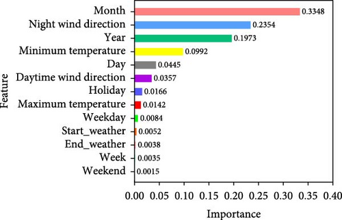
Based on the actual situation, we set the threshold of feature importance score to 0.005 and delete the features with scores lower than 0.005, that is, end_weather, Week, and Weekend. Retain 10 characteristic variables: Month, Night wind direction, Year, Minimum temperature, Day, Daytime wind direction, Holiday, Maximum temperature, Weekday, and Start_weather.

4. Evaluation Metrics

4.1. Point Prediction Evaluation Metrics

For a single point prediction, the mean absolute error (MAE), root mean square error (RMSE), mean absolute percentage error (MAPE), and goodness of fit (R²) are selected to evaluate the prediction accuracy of the model in this paper, which is calculated as follows:

()

where t is the number of samples, y_t is the real load value at time t, y_e,t is the predicted load value at time t, and

is the average of all real values. Among the above indicators, the smaller the value of MAE, RMSE, and MAPE, the better the prediction effect of the model; the larger the value of R², the better the prediction effect of the model.

4.2. Interval Prediction Evaluation Metrics

In the context of interval prediction, two metrics are commonly used to assess the quality of prediction intervals: prediction interval coverage probability (PICP) and prediction interval normalized averaged width (PINAW). PICP measures the probability that the true value falls within the upper and lower bounds of the prediction interval. A higher PICP indicates a better prediction accuracy, as it signifies a greater likelihood of the prediction interval containing the true value. PINAW, on the other hand, quantifies the average width of the prediction interval. The lower the PINAW value, the more effective the model’s prediction. These two indicators are calculated as follows:

()

where I_t is the Boolean variable, y_t is the actual value of the power load, L_t is the lower bound of the forecast interval, U_t is the upper bound of the forecast interval, and R is the range between the actual values.

4.3. Probability Prediction Evaluation Metrics

For probabilistic prediction evaluation, we utilize the average pinball loss (APL) and continuous ranked probability score (CRPS) as metrics to assess the effectiveness of the model’s probabilistic predictions. APL represents the average value of the pinball loss and functions as the model’s loss function. A smaller APL value indicates better prediction performance of the model, and it is calculated as shown in Equation (12). CRPS measures the discrepancy between the predicted distribution and the true distribution through quadrature. It is used to compare a single true value with its predicted distribution. Its calculation formula is as follows:

()

where CDF(⋅) is the cumulative distribution function of the load forecast value and H(⋅) is the step function, whose value is 1 when y_t > y_e,t and 0 when y_t ≤ y_e,t. CRPS comprehensively considers the complete probability distribution of the load forecast value. The lower the value, the closer the model’s probability prediction result is to the distribution of the actual value, indicating a better prediction performance.

5. IFS-GA-QRLSTM

5.1. Introduction

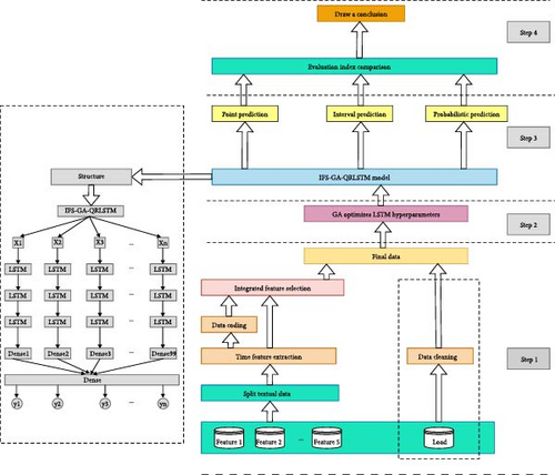
This paper proposes a new hybrid probabilistic prediction model, IFS-GA-QRLSTM, to address the lack of research in load probability forecasting and variable feature screening methods. The model begins by employing an integrated feature selection algorithm to identify the 10 most relevant features for load data. The data are then divided into training and test sets, with 80% used for training and 20% for testing. To optimize the model parameters automatically, a genetic algorithm is utilized to determine the number of LSTM layers, dense layers, hidden layer neurons, and dense layer neurons. The model integrates LSTM with quantile regression to generate point, interval, and probability predictions. The results are comprehensively analyzed to draw conclusions. The structural design of the model is illustrated in Figure 9.

5.2. Experimental Setup

(1)
Hyperparameter settings for IFS-GA-QRLSTM and baseline models

In the implementation of deep learning tasks, the selection of parameters plays a crucial role in determining the training accuracy of the model. Table 3 provides a detailed comparison of the parameter configurations between the IFE-GA-QRLSTM model and the baseline models.

Table 3. Hyperparameters of IFS-GA-QRLSTM and baseline models.

Algorithm	Hyperparameter	Value
IFS-GA-QRLSTM and baseline models	Time_step	96
	Batch size	32
	Number of LSTM layers	2
	Number of dense layers	1
	LSTM units	30
	Dense units	64
	Optimizer	Adam
	Learning rate	0.005
	Epochs	150
	Loss function	Pinball loss
	Activation function	relu, tanh
	Dropout	0.1

(2)
Hyperparameter setting of GA

The accuracy of a genetic algorithm is primarily determined by parameters such as DNA_size, DNA_size_max, POP_size, Cross_rate, Mutation_rate, and N_generations. When applying a genetic algorithm to optimize LSTM hyperparameters, it is important to consider that increasing the number of LSTM layers can lead to higher computational costs for the prediction model. Some studies have utilized a two-layer LSTM network structure to improve the predictive performance of time series data. However, it has been noted in literature that exceeding three layers in an LSTM network may result in significant gradient vanishing issues between layers. Therefore, the design of deep LSTM network structures typically restricts the number of LSTM layers to 1–3, with the number of neurons in the hidden layer falling within the (32, 256) range. The hyperparameters of the genetic algorithm are outlined in Table 4.

Table 4. Hyperparameters of GA.

Algorithm	Hyperparameter	Value
GA	DNA_size	2
	DNA_size_max	8
	POP_size	20
	Cross_rate	0.5
	Mutation_rate	0.01
	N_generations	20

(3)
The parameter results after GA optimization

In this paper, GA will optimize the number of LSTM layers, dense layers, hidden layer neurons, and dense layer neurons. The optimized results are displayed in Table 5.

Table 5. Comparison of hypeparameters before and after GA optimization.

Optimized hyperparameter	Before	After
Number of LSTM layers	2	3
LSTM units	30, 30	82, 175, 67
Number of dense layers	1	1
Dense units	64	94

The above optimization results were obtained by finding out the gene corresponding to the chromosome with the greatest fitness, where the maximum fitness was 3,489.7931. It can be observed from the table that the number of layers in the optimized LSTM becomes three layers, and the dense layer is still one layer, but the number of hidden neurons has significant changes. Next, we will adjust the parameters of the IFE-QRLSTM model based on the above optimization results and then carry out the subsequent case analysis.

5.3. Experimental Environment

The experimental setup for this study involved using PyCharm interpreter, Python 3.8, and TensorFlow 2.6 GPU versions to develop a short-term power load probability prediction model for campus users. The model was built using the TensorFlow and Keras frameworks.

5.4. Experimental Analysis and Evaluation

5.4.1. Point Prediction

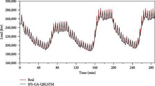
For a single point prediction, we use the previous day’s data, namely, 96 data points, to predict the load data of the next moment, and take the output of the model with a quantile of 0.5 as the output of the actual point prediction. Figure 10 shows the forecast results of the first 3 days of the IFS-GA-QRLSTM model.

In order to further validate the predictive performance of the IFS-GA-QRLSTM model, we selected five basic models, namely, QRLSTM, IFS-QRCNN, IFS-QRRNN, IFS-QRGRU, and IFS-QRLSTM, and compared them with IFS-GA-QRLSTM. QRLSTM represents the model that combines LSTM with quantile regression. IFS-QRLSTM represents the model that first performs integrated feature selection on the data and then combines LSTM with quantile regression. IFE-GA-QRLSTM represents the model that first performs integrated feature selection on the data, then optimizes the hyperparameters of LSTM using a genetic algorithm, and finally combines it with quantile regression to form the final model. The other comparison models are similar to the ones mentioned above. The prediction results of different models are shown in Figure 11.

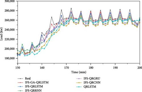
The figure illustrates that the prediction results of the IFS-GA-QRLSTM model are more closely aligned with the true value curve when compared to the other models. In order to show the prediction errors of different models more clearly, we compare the above models in detail through the four-point prediction evaluation indexes of MAE, RMSE, MAPE, and R², and the results are shown in Table 6.

Table 6. Assessment results of point prediction.

Index	QRLSTM	IFS-QRCNN	IFS-QRRNN	IFS-QRGRU	IFS-QRLSTM	IFS-GA-QRLSTM
MAE	7,217.7585	6,739.1801	5,639.9237	4,889.7566	2,752.7269	2,155.0767
RMSE	10,360.6550	9,365.1681	8,030.5217	7,052.9051	5,767.0652	5,070.7624
MAPE	3.7857	3.4566	3.1002	2.4861	1.6245	1.3408
R²	0.8964	0.9153	0.9377	0.9520	0.9679	0.9752

It can be clearly seen from the table that the prediction effect of IFS-GA-QRLSTM model is the best, followed by IFS-QRLSTM, IFS-QRGRU, IFS-QRRNN, IFS-QRCNN, and QRLSTM. The R² of IFS-GA-QRLSTM model reached 0.9752, which was increased by 0.75%, 2.44%, 4.00%, 6.54%, and 8.79% compared with IFS-QRLSTM, IFS-QRGRU, IFS-QRRNN, IFS-QRCNN, and QRLSTM models, respectively. The MAE is 2155.0767, which is decreased by 21.71%, 55.93%, 61.79%, 68.02%, and 70.14% compared with the above five models. The RMSE was 5070.7624, which was decreased by 12.07%, 28.10%, 36.86%, 45.86%, and 51.06% compared with the above five models. Its MAPE value was 1.3408, which was reduced by 17.46%, 46.07%, 56.75%, 61.21%, and 64.58% compared with the above five models. The superior point prediction results of the IFS-GA-QRLSTM model demonstrate the effectiveness and efficiency of the integrated feature selection algorithm proposed in this paper.

5.4.2. Interval Prediction

For interval prediction, we will continue to use the dataset mentioned above to predict the data for the next time interval based on the data from the previous day. However, different from point prediction, interval prediction can give the predicted value under different quantile at the next moment. In this paper, the quantile value interval is set as (0.01, 0.99), with a quantile interval of 0.01. Therefore, there are a total of 99 quantiles. That is, the value of 99 quantiles at the next moment is predicted, and the 0.05 quantile is used as the lower bound of the prediction interval, the 0.95 quantile is used as the upper bound of the prediction interval, and the prediction interval of 90% of the predicted value is given. The interval prediction results of IFS-GA-QRLSTM model and 90% of the above five comparison models are shown in Figure 12.

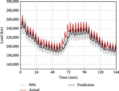
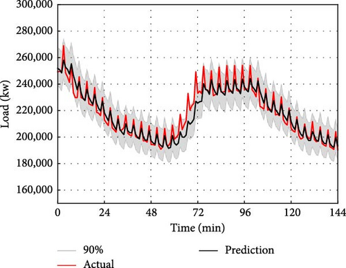
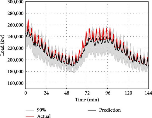
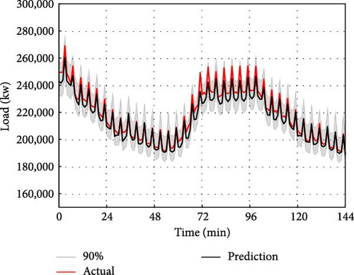
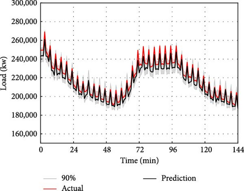
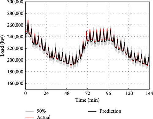
The interval prediction effect of the IFS-GA-QRLSTM model is superior to that of other basic models as depicted in the figure. This is evident from the narrow interval bandwidth and the prediction interval which almost fully encompasses the actual value. To provide a clearer description of the prediction performance of the IFS-GA-QRLSTM model, this paper utilizes the evaluation indicators of PICP and PINAW for interval prediction analysis. The evaluation index pairs for the aforementioned model are presented in Table 7.

Table 7. Assessment results of interval prediction.

Index	QRLSTM	IFS-QRCNN	IFS-QRRNN	IFS-QRGRU	IFS-QRLSTM	IFS-GA-QRLSTM
PICP	0.8575	0.9319	0.9442	0.9515	0.9636	0.9947
PINAW	0.0833	0.1101	0.0962	0.0767	0.0612	0.0439

The table clearly shows that the IFS-GA-QRLSTM model outperforms others in terms of the two evaluation indicators mentioned, followed by IFS-QRLSTM, IFS-QRGRU, IFS-QRRNN, IFS-QRCNN, and QRLSTM. The PICP of the IFS-GA-QRLSTM model reached 0.9947, and the coverage rate of the prediction interval reached the highest, which was increased by 3.23%, 4.54%, 5.35%, 6.74%, and 16% compared with the above five models. PINAW is 0.0439, which is the narrowest interval width compared with the other five basic models, and decreased by 28.27%, 42.76%, 54.37%, 60.13%, and 47.30% compared with the above four models, respectively. Therefore, it can be shown that the IFS-GA-QRLSTM model still performs best in interval prediction.

5.4.3. Probabilistic Prediction

For probabilistic prediction, we still use the above dataset to predict the next moment through the load data of the previous day. Unlike point and interval prediction, probabilistic prediction can be done by taking the 99 quantile values of the predicted point and inputting them into the kernel density estimation as a set of random variables, which gives the probability density function of that predicted point. Figure 13 illustrates the probabilistic prediction results at the 81st point for the six models described above.

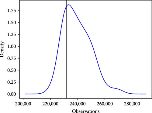
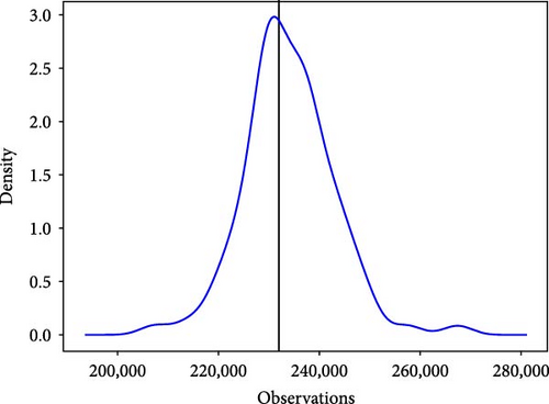
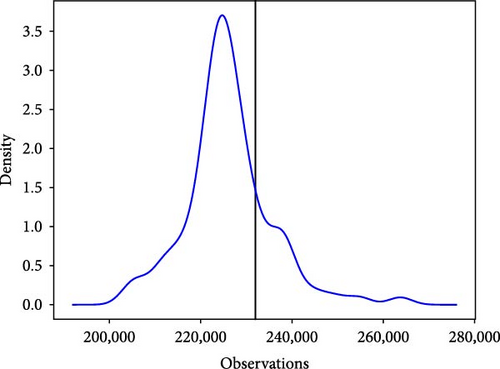
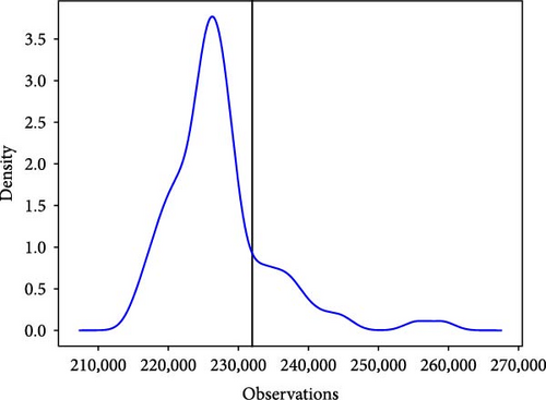
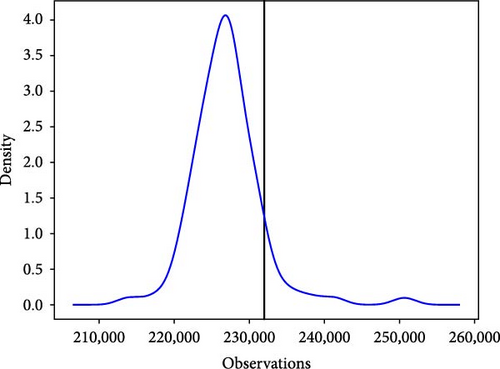
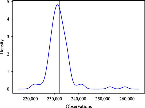
The black vertical line in the figure above represents the true value of the 81st point, and the red curve represents the probability density function of the point. It can be observed from the probability density function diagram that the true values of the six models fall within the curve and are relatively close to its highest point. Among the six basic models, the IFS-GA-QRLSTM model stands out as its peak value aligns closely with the actual load value, exhibiting the highest density at this point and the most stable curve. This further indicates that the IFS-GA-QRLSTM model performs better in probability prediction compared to the other five models.

Similarly, to better compare the predictive performance of different models, we use APL and CRPS to further evaluate the aforementioned models. Figure 14 presents the comparison results of evaluation indexes of the five models.

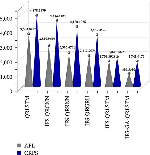
The IFS-GA-QRLSTM model exhibits the smallest APL and CRPS values among the models shown in the figure, indicating that its predicted values are closest to the actual values. This suggests that the model has the smallest prediction error and the best predictive performance. It is followed by IFS-QRLSTM, IFS-QRGRU, IFS-QRRNN, IFS-QRCNN, and QRLSTM. The APL value of IFS-GA-QRLSTM model was 881.3393, which decreased by 49.71%, 58.31%, 61.74%, 68.75%, and 75.58%, respectively, compared with the above five models. The CRPS value was 1741.6173, which was decreased by 13.87%, 50.70%, 57.73%, 61.66%, and 64.30%, respectively, compared with the above five models. Therefore, it has been demonstrated that the IFS-GA-QRLSTM model has the best predictive performance, significantly reducing prediction errors compared to other models.

6. Conclusions

Regional short-term load probability prediction plays a crucial role in power dispatching within power systems and energy management. In this study, a novel hybrid model, IFS-GA-QRLSTM, is proposed and evaluated in terms of point prediction, interval prediction, and probability prediction. It is compared against five basic models: IFS-QRLSTM, IFS-QRGRU, IFS-QRRNN, IFS-QRCNN, and QRLSTM. Results indicate that the IFS-GA-QRLSTM model outperforms the others, demonstrating the smallest prediction error and the best forecasting effect, affirming the superiority of the proposed approach. As technology advances, new methods will continue to enhance power load forecasting accuracy to meet diverse needs. While this study shows promising results, it still lacks in certain aspects. Future research should explore the application of the proposed method in medium- and long-term load probability prediction, investigate additional combined forecasting models, conduct comprehensive comparative tests, and identify the optimal model to enhance the stability of load probability prediction.

Conflicts of Interest

The authors have no conflicts of interest to declare.

Acknowledgments

This work has been supported by the Shangdong Province Social Science Planning and Research Project (no. 23CSDJ12).

Open Research

Data Availability

The power load data used to support the findings of this study were supplied by a regional power grid company in Yantai under license and so cannot be made freely available. Requests for access to these data should be made to Xigao Shao, [email protected].

References

1 Gigoni L., Betti A., Crisostomi E., Franco A., Tucci M., Bizzarri F., and Mucci D., Day-ahead hourly forecasting of power generation from photovoltaic plants, IEEE Transactions on Sustainable Energy. (2018) 9, no. 2, 831–842, https://doi.org/10.1109/TSTE.2017.2762435, 2-s2.0-85031765425.
10.1109/TSTE.2017.2762435
Web of Science® Google Scholar
2 Jinjin Z., Qian Z., Guoli L., Yuan M., and Can W., Application of HIMVO-SVM in short-term load forecasting, 2020 Chinese Control And Decision Conference (CCDC), 2020, IEEE, 768–772.
Google Scholar
3 Yang W., Jia L., and Xu Y., Adaptive data decomposition based quantile-long-short-term memory probabilistic forecasting framework for power demand side management of energy system, Computers and Electrical Engineering. (2023) 106, https://doi.org/10.1016/j.compeleceng.2023.108584, 108584.
10.1016/j.compeleceng.2023.108584
Web of Science® Google Scholar
4 Yuan X., Chen C., Jiang M., and Yuan Y., Prediction interval of wind power using parameter optimized Beta distribution based LSTM model, Applied Soft Computing. (2019) 82, https://doi.org/10.1016/j.asoc.2019.105550, 2-s2.0-85066951367, 105550.
10.1016/j.asoc.2019.105550
Web of Science® Google Scholar
5 Wang Z., Li H., Tang Z., and Liu Y., User-level ultra-short-term load forecasting model based on optimal feature selection and bahdanau attention mechanism, Journal of Circuits, Systems and Computers. (2021) 30, no. 15, https://doi.org/10.1142/S0218126621502790, 2150279.
10.1142/S0218126621502790
Web of Science® Google Scholar
6 Li H., Liu H., Ji H., Zhang S., and Li P., Ultra-short-term load demand forecast model framework based on deep learning, Energies. (2020) 13, no. 18, https://doi.org/10.3390/en13184900, 4900.
10.3390/en13184900
Web of Science® Google Scholar
7 Feihong L. and Yingqun X., Short-term power load forecasting method based on VMD-GRU-EC, China Test and Technology. (2023) 49, no. 10, 120–127.
Google Scholar
8 Shang Z., He Z., Song Y., Yang Y., Li L., and Chen Y., A novel combined model for short-term electric load forecasting based on whale optimization algorithm, Neural Processing Letters. (2020) 52, no. 2, 1207–1232, https://doi.org/10.1007/s11063-020-10300-0.
10.1007/s11063-020-10300-0
Web of Science® Google Scholar
9 Li L.-L., Sun J., Wang C.-H., Zhou Y.-T., and Lin K.-P., Enhanced Gaussian process mixture model for short-term electric load forecasting, Information Sciences. (2019) 477, 386–398, https://doi.org/10.1016/j.ins.2018.10.063, 2-s2.0-85055914795.
10.1016/j.ins.2018.10.063
Web of Science® Google Scholar
10 ZulfiqAr M., Kamran M., Rasheed M. B., Alquthami T., and Milyani A. H., A short-term load forecasting model based on self-adaptive momentum factor and wavelet neural network in smart grid, IEEE Access. (2022) 10, 77587–77602, https://doi.org/10.1109/ACCESS.2022.3192433.
10.1109/ACCESS.2022.3192433
Web of Science® Google Scholar
11 Pedregal D. J. and Trapero J. R., Mid-term hourly electricity forecasting based on a multi-rate approach, Energy Conversion and Management. (2010) 51, no. 1, 105–111, https://doi.org/10.1016/j.enconman.2009.08.028, 2-s2.0-74249107853.
10.1016/j.enconman.2009.08.028
Web of Science® Google Scholar
12 Bouktif S., Fiaz A., Ouni A., and Serhani M. A., Single and multi-sequence deep learning models for short and medium term electric load forecasting, Energies. (2019) 12, no. 1, https://doi.org/10.3390/en12010149, 2-s2.0-85060028261, 149.
10.3390/en12010149
Web of Science® Google Scholar
13 Carvallo J. P., Larsen P. H., Sanstad A. H., and Goldman C. A., Long term load forecasting accuracy in electric utility integrated resource planning, Energy Policy. (2018) 119, 410–422, https://doi.org/10.1016/j.enpol.2018.04.060, 2-s2.0-85046726700.
10.1016/j.enpol.2018.04.060
Web of Science® Google Scholar
14 Lindberg K. B., Bakker S. J., and Sartori I., Modelling electric and heat load profiles of non-residential buildings for use in long-term aggregate load forecasts, Utilities Policy. (2019) 58, 63–88, https://doi.org/10.1016/j.jup.2019.03.004, 2-s2.0-85064915699.
10.1016/j.jup.2019.03.004
Web of Science® Google Scholar
15 Lindberg K. B., Seljom P., Madsen H., Fischer D., and Korpås M., Long-term electricity load forecasting: current and future trends, Utilities Policy. (2019) 58, 102–119, https://doi.org/10.1016/j.jup.2019.04.001, 2-s2.0-85065077619.
10.1016/j.jup.2019.04.001
Web of Science® Google Scholar
16 Dongfeng C., Zhou Z., and Yongfeng W., Analysis of short-term load forecasting problem of power system based on time series, Automation Application. (2017) 11, 99–101.
Google Scholar
17 Sharma S., Majumdar A., Elvira V., and Chouzenoux É., Blind Kalman filtering for short-term load forecasting, IEEE Transactions on Power Systems. (2020) 35, no. 6, 4916–4919, https://doi.org/10.1109/TPWRS.59, 2-s2.0-85042656116.
10.1109/TPWRS.2020.3018623
Web of Science® Google Scholar
18 Mi J., Fan L., Duan X., and Qiu Y., Short-term power load forecasting method based on improved exponential smoothing grey model, Mathematical Problems in Engineering. (2018) 2018, 11, https://doi.org/10.1155/2018/3894723, 2-s2.0-85045547104, 3894723.
10.1155/2018/3894723
Web of Science® Google Scholar
19 Saber A. Y. and Alam A. K. M. R., Short term load forecasting using multiple linear regression for big data, 2017 IEEE Symposium Series on Computational Intelligence (SSCI), 2017, IEEE, 1–6.
Google Scholar
20 Singh U. and Vadhera S., Random forest and xgboost technique for short-term load forecasting, 1st International Conference on Sustainable Technology for Power and Energy Systems (STPES), 2022, IEEE, 1–6.
Google Scholar
21 Kong W., Dong Z. Y., Jia Y., Hill D. J., Xu Y., and Zhang Y., Short-term residential load forecasting based on LSTM recurrent neural network, IEEE Transactions on Smart Grid. (2019) 10, no. 1, 841–851, https://doi.org/10.1109/TSG.2017.2753802, 2-s2.0-85030636120.
10.1109/TSG.2017.2753802
Web of Science® Google Scholar
22 Aslam S., Herodotou H., Mohsin S. M., Javaid N., Ashraf N., and Aslam S., A survey on deep learning methods for power load and renewable energy forecasting in smart microgrids, Renewable and Sustainable Energy Reviews. (2021) 144, https://doi.org/10.1016/j.rser.2021.110992, 110992.
10.1016/j.rser.2021.110992
Web of Science® Google Scholar
23 Giacomazzi E., Haag F., and Hopf K., Short-term electricity load forecasting using the temporal fusion transformer: effect of grid hierarchies and data sources, The 14th ACM International Conference on Future Energy Systems, 2023, Orlando, FL, USA, 353–360.
Google Scholar
24 Hopf K., Hartstang H., and Staake T., Meta-regression analysis of errors in short-term electricity load forecasting, Companion Proceedings of the 14th ACM International Conference on Future Energy Systems, 2023, New York, NY, USA, 32–39.
Google Scholar
25 Haben S., Arora S., Giasemidis G., Voss M., and Vukadinović Greetham D., Review of low voltage load forecasting: methods, applications, and recommendations, Applied Energy. (2021) 304, https://doi.org/10.1016/j.apenergy.2021.117798, 117798.
10.1016/j.apenergy.2021.117798
Web of Science® Google Scholar
26 Xie J. and Hong T., GEFCom2014 probabilistic electric load forecasting: an integrated solution with forecast combination and residual simulation, International Journal of Forecasting. (2016) 32, no. 3, 1012–1016, https://doi.org/10.1016/j.ijforecast.2015.11.005, 2-s2.0-84950126041.
10.1016/j.ijforecast.2015.11.005
Web of Science® Google Scholar
27 Xu L., Wang S., and Tang R., Probabilistic load forecasting for buildings considering weather forecasting uncertainty and uncertain peak load, Applied Energy. (2019) 237, 180–195, https://doi.org/10.1016/j.apenergy.2019.01.022, 2-s2.0-85059570431.
10.1016/j.apenergy.2019.01.022
Web of Science® Google Scholar
28 Wang Y., Zhang N., Tan Y., Hong T., Kirschen D. S., and Kang C., Combining probabilistic load forecasts, IEEE Transactions on Smart Grid. (2018) 10, no. 4, 3664–3674, https://doi.org/10.1109/TSG.5165411.
10.1109/TSG.2018.2833869
Web of Science® Google Scholar
29 Dengwu Yu, Min Liu, and Fanuo Pu, Load interval forecasting method based on deep learning quantile regression, Guangdong Electric Power. (2022) 35, no. 9, 1–8.
Google Scholar
30 Wentao Z., Guangtao W., and Zeli W., User-level short-term load probability forecasting method for night economy based on LightGBM, Frontiers in Data and Computing. (2019) 5, no. 3, 160–168.
Google Scholar
31 Wang Y., Gan D., Sun M., Zhang N., Lu Z., and Kang C., Probabilistic individual load forecasting using pinball loss guided LSTM, Applied Energy. (2019) 235, 10–20, https://doi.org/10.1016/j.apenergy.2018.10.078, 2-s2.0-85055915128.
10.1016/j.apenergy.2018.10.078
Web of Science® Google Scholar
32 Jinyang Li, Research on short-term load probability prediction based on Copula and nonlinear quantile regression, 2022, Hunan Normal University, MS thesis.
Google Scholar
33 Wei Z., Chengbo Y. U., and Shibin W., Multi-feature short-term power load forecasting based on VMD-LSTM-LightGBM, China Southern Power Grid Technology. (2023) 17, no. 2, 74–81, https://doi.org/10.13648/j.cnki.issn1674-0629.2023.02.009.
10.13648/j.cnki.issn1674-0629.2023.02.009
Google Scholar
34 Jiang H. and Zheng W., Deep learning with regularized robust long-and short-term memory network for probabilistic short-term load forecasting, Journal of Forecasting. (2022) 41, no. 6, 1201–1216, https://doi.org/10.1002/for.2855.
10.1002/for.2855
Web of Science® Google Scholar
35 Yue X. I. E., Liang R., and Liang Z., Attention-based dense LSTM for speech emotion recognition, The Institute of Electronics, Information and Communication Engineers. (2019) 500, no. 7, E102.
Google Scholar
36 Ma H., Peng T., Zhang C., Ji C., Li Y., and Nazir M. S., Developing an evolutionary deep learning framework with random forest feature selection and improved flow direction algorithm for NOx concentration prediction, Engineering Applications of Artificial Intelligence. (2023) 123, https://doi.org/10.1016/j.engappai.2023.106367, 106367.
10.1016/j.engappai.2023.106367
Web of Science® Google Scholar
37 Wang Y., Sun S., Chen X., Zeng X., Kong Y., Chen J., Guo Y., and Wang T., Short-term load forecasting of industrial customers based on SVMD and XGBoost, International Journal of Electrical Power & Energy Systems. (2021) 129, https://doi.org/10.1016/j.ijepes.2021.106830, 106830.
10.1016/j.ijepes.2021.106830
Web of Science® Google Scholar
38 Zeming L. I. and Daling Z., Daily gas load prediction based on XGB-LSTM model, City Gas. (2023) 11, 22–27.
Google Scholar
39 Wang Y., Chen J., Chen X., Zeng X., Kong Y., Sun S., Guo Y., and Liu Y., Short-term load forecasting for industrial customers based on TCN-LightGBM, IEEE Transactions on Power Systems. (2020) 36, no. 3, 1984–1997.
10.1109/TPWRS.2020.3028133
Web of Science® Google Scholar
40 Tian L., Feng L., Yang L., and Guo Y., Stock price prediction based on LSTM and LightGBM hybrid model, The Journal of Supercomputing. (2022) 78, no. 9, 11768–11793, https://doi.org/10.1007/s11227-022-04326-5.
10.1007/s11227-022-04326-5
Web of Science® Google Scholar
41 Bouktif S., Fiaz A., Ouni A., and Serhani M. A., Optimal deep learning LSTM model for electric load forecasting using feature selection and genetic algorithm: comparison with machine learning approaches, Energies. (2018) 11, no. 7, https://doi.org/10.3390/en11071636, 2-s2.0-85051226929, 1636.
10.3390/en11071636
Web of Science® Google Scholar
42 Jingyi Li, Fei D., Zhang Nan L. I. X., and Chao G. U., Short-term traffic flow prediction model based on fusion of deep LSTM and genetic algorithm, Radio Communication Technology. (2022) 48, no. 5, 836–843.
Google Scholar
43 Jiajia Z. and Dingsheng W., Study on flow prediction of small and medium watershed based on mixed GA optimization LSTM, Computer. (2022) 39, no. 2, 283–287 342.
Google Scholar
44 Wu K., Wu J., Feng L., Yang B., Liang R., Yang S., and Zhao R., An attention-based CNN-LSTM-BiLSTM model for short-term electric load forecasting in integrated energy system, International Transactions on Electrical Energy Systems. (2021) 31, no. 1, https://doi.org/10.1002/2050-7038.12637, e12637.
10.1002/2050-7038.12637
Web of Science® Google Scholar
45 Hansun S. and Young J. C., Predicting LQ45 financial sector indices using RNN-LSTM, Journal of Big Data. (2021) 8, no. 1, 1–13, https://doi.org/10.1186/s40537-021-00495-x.
10.1186/s40537-021-00495-x
PubMed Web of Science® Google Scholar
46 Cascone L., Sadiq S., Ullah S., Mirjalili S., Siddiqui H. U. R., and Umer M., Predicting household electric power consumption using multi-step time series with convolutional LSTM, Big Data Research. (2023) 31, https://doi.org/10.1016/j.bdr.2022.100360, 100360.
10.1016/j.bdr.2022.100360
Web of Science® Google Scholar
47 Duan Y., A novel interval energy-forecasting method for sustainable building management based on deep learning, Sustainability. (2022) 14, no. 14, https://doi.org/10.3390/su14148584, 8584.
10.3390/su14148584
Web of Science® Google Scholar

Citing Literature

All articles

Short-Term Load Probability Prediction Based on Integrated Feature Selection and GA-LSTM Quantile Regression

Abstract

1. Introduction

1.1. Background of the Study

1.2. Literature Reviews

1.3. Contributions

2. Methodologies

2.1. Integrated Feature Selection

2.2. GA

2.3. LSTM

2.4. Probabilistic Prediction Model

3. Data Preprocessing

3.1. Dataset Introduction

3.2. Missing and Outlier Processing and Data Standardization

3.3. Time-Dependent Feature Extraction and Coding

3.4. Integrated Feature Selection

4. Evaluation Metrics

4.1. Point Prediction Evaluation Metrics

4.2. Interval Prediction Evaluation Metrics

4.3. Probability Prediction Evaluation Metrics

5. IFS-GA-QRLSTM

5.1. Introduction

5.2. Experimental Setup

5.3. Experimental Environment

5.4. Experimental Analysis and Evaluation

5.4.1. Point Prediction

5.4.2. Interval Prediction

5.4.3. Probabilistic Prediction

6. Conclusions

Conflicts of Interest

Acknowledgments

Open Research

Data Availability

References

Citing Literature

Figures

References

Related

Information