International Journal of Energy Research

Volume 2024, Issue 1 5198814

Research Article

Open Access

Islanding Detection and Power Quality Diagnosis of Wind Power Integrated Microgrid with Reduced Feature Trained Novel Optimized Random Decision Forest

Sairam Mishra,

Sairam Mishra

orcid.org/0009-0005-8612-7209

Department of Electrical Engineering, Siksha ‘O’ Anushandhan Deemed to Be University, Bhubaneswar, India

Search for more papers by this author

Ranjan K. Mallick,

Ranjan K. Mallick

orcid.org/0000-0003-0375-6551

Department of Electrical and Electronics Engineering, Siksha ‘O’ Anushandhan Deemed to Be University, Bhubaneswar, India

Search for more papers by this author

Debadatta A. Gadanayak,

Debadatta A. Gadanayak

orcid.org/0000-0001-7533-4441

Department of Electrical and Electronics Engineering, Siksha ‘O’ Anushandhan Deemed to Be University, Bhubaneswar, India

Search for more papers by this author

Pravati Nayak,

Pravati Nayak

orcid.org/0009-0004-1303-7889

Department of Electrical Engineering, Siksha ‘O’ Anushandhan Deemed to Be University, Bhubaneswar, India

Search for more papers by this author

Aymen Flah,

Aymen Flah

orcid.org/0000-0002-3463-6096

Energy Processes Environment and Electrical Systems Unit, National Engineering School of Gabès, University of Gabes, Gabès 6029, Tunisia univgb.rnu.tn

University of Business and Technology (UBT), College of Engineering, Jeddah 21448, Saudi Arabia ubt.edu.sa

MEU Research Unit, Middle East University, Amman 11831, Jordan meu.edu.jo

University of Gabès, Private Higher School of Applied Sciences and Technology of Gabès, Gabès 6029, Tunisia univgb.rnu.tn

ENET Centre, VSB-Technical University of Ostrava, Ostrava, Czech Republic vsb.cz

Applied Science Research Center, Applied Science Private University, Amman 11931, Jordan asu.edu.jo

Search for more papers by this author

Claude Ziad El-Bayeh,

Claude Ziad El-Bayeh

orcid.org/0000-0002-8268-8878

Department of Electrical Engineering, Bayeh Institute, 55 Kfar Saleh-Hay El Arbe Street, Amchit, Mount Lebanon, Lebanon

Search for more papers by this author

Habib Kraiem,

Corresponding Author

Habib Kraiem

[email protected]

orcid.org/0000-0003-3248-2430

Department of Electrical Engineering, College of Engineering, Northern Border University, Arar, Saudi Arabia nbu.edu.sa

Search for more papers by this author

Lukas Prokop,

Lukas Prokop

orcid.org/0000-0003-0495-5499

ENET Centre, VSB-Technical University of Ostrava, Ostrava, Czech Republic vsb.cz

Search for more papers by this author

Sairam Mishra,

Sairam Mishra

orcid.org/0009-0005-8612-7209

Department of Electrical Engineering, Siksha ‘O’ Anushandhan Deemed to Be University, Bhubaneswar, India

Search for more papers by this author

Ranjan K. Mallick,

Ranjan K. Mallick

orcid.org/0000-0003-0375-6551

Department of Electrical and Electronics Engineering, Siksha ‘O’ Anushandhan Deemed to Be University, Bhubaneswar, India

Search for more papers by this author

Debadatta A. Gadanayak,

Debadatta A. Gadanayak

orcid.org/0000-0001-7533-4441

Department of Electrical and Electronics Engineering, Siksha ‘O’ Anushandhan Deemed to Be University, Bhubaneswar, India

Search for more papers by this author

Pravati Nayak,

Pravati Nayak

orcid.org/0009-0004-1303-7889

Department of Electrical Engineering, Siksha ‘O’ Anushandhan Deemed to Be University, Bhubaneswar, India

Search for more papers by this author

Aymen Flah,

Aymen Flah

orcid.org/0000-0002-3463-6096

Energy Processes Environment and Electrical Systems Unit, National Engineering School of Gabès, University of Gabes, Gabès 6029, Tunisia univgb.rnu.tn

University of Business and Technology (UBT), College of Engineering, Jeddah 21448, Saudi Arabia ubt.edu.sa

MEU Research Unit, Middle East University, Amman 11831, Jordan meu.edu.jo

University of Gabès, Private Higher School of Applied Sciences and Technology of Gabès, Gabès 6029, Tunisia univgb.rnu.tn

ENET Centre, VSB-Technical University of Ostrava, Ostrava, Czech Republic vsb.cz

Applied Science Research Center, Applied Science Private University, Amman 11931, Jordan asu.edu.jo

Search for more papers by this author

Claude Ziad El-Bayeh,

Claude Ziad El-Bayeh

orcid.org/0000-0002-8268-8878

Department of Electrical Engineering, Bayeh Institute, 55 Kfar Saleh-Hay El Arbe Street, Amchit, Mount Lebanon, Lebanon

Search for more papers by this author

Habib Kraiem,

Corresponding Author

Habib Kraiem

[email protected]

orcid.org/0000-0003-3248-2430

Department of Electrical Engineering, College of Engineering, Northern Border University, Arar, Saudi Arabia nbu.edu.sa

Search for more papers by this author

Lukas Prokop,

Lukas Prokop

orcid.org/0000-0003-0495-5499

ENET Centre, VSB-Technical University of Ostrava, Ostrava, Czech Republic vsb.cz

Search for more papers by this author

First published: 29 March 2024

https://doi.org/10.1155/2024/5198814

Citations: 3

Academic Editor: Longxing Wu

Share a link

Email
Wechat
Bluesky

Abstract

Distributed generations (DGs) have been increasingly addressing the ongoing power deficit in the electricity market. However, a significant concern in DG-integrated microgrids is the detection of accidental islanding. To tackle this issue, this article proposes a cost-friendly, novel data-driven passive islanding detection scheme named EEMD-HOBRC, combining noise-assisted ensemble empirical mode decomposition (EEMD) and a hybrid optimization-based random forest classifier (HOBRFC). The detection scheme employs a diverse set of features extracted from both raw and EEMD decomposed signals. Essential features are selected using the binary grey wolf optimizer (BGWO) to reduce computational burden. To further improve classification accuracy, the parameters of the random forest classifier are optimized through a hybrid particle swarm and reformed grey wolf optimization (PSRGWO) technique with Cohen’s kappa index as the cost function. The proposed technique is rigorously validated in two different multi-DG environments, encompassing islanding and various nonislanding events. The results demonstrate the effectiveness of the approach in terms of enhanced accuracy, detection time, and performance under both noisy and noise-free conditions. The accuracy of detection under ideal and high noise scenarios is found to be 99.88% and 99.2%, respectively, with maximum detection time of 34.27 ms. Comparative analysis with other algorithms also supports the superiority of the proposed technique. Finally, the method is successfully applied to shrink the nondetection zone (NDZ) with minimal power mismatch, further enhancing its utility in practical applications.

1. Introduction

Distributed generators (DGs) are proving to be the best solution to match the ongoing demand for electricity. Since every solution is equipped with new problem(s), the DGs are equipped with the challenge of unintentional islanding. In simple terms, islanding is such a scenario where the DG(s) of an area is/are kept on supplying power to the nearby loads even though the central grid is no longer connected. This occurrence should be detected within 2 sec as per IEEE 1547 [1] norms. The conventional strategies of islanding detection [2–5] have a common concern that is reducing the nondetection zone (NDZ). By definition, NDZ is a power mismatch region where the islanding is remained undetected due to supply-demand equilibrium. Several research works have already proposed to conquer the NDZ issue by applying signal processing approach (SPA) to the conventional passive detection techniques [6, 7]. But still, these have issues like computational complexity, affected by noise interference, and unapplicable to nonlinear and nonstationary signals. Hence, the necessity of further research is essential in this particular field. Eventually, mode decomposition- (MD-) oriented SPAs are gaining popularity that brings forward empirical MD (EMD) [8], variational MD (VMD) [9], and empirical wavelet transform (EWT) [10] into the limelight. But these MD techniques basically suffer from mode mixing issues. This major drawback is wonderfully eliminated by a recently proposed noise-assisted technique called ensemble EMD (EEMD) [11] by taking the mean of an aggregate of trials that comprises of signal and finite amplitude white noise. It has also displayed significant results in detecting differential protection [12], load forecasting [13], wind speed prediction [14], etc. Thus, EEMD is chosen as the base SPA in this work.

Disturbance detection only with SPA brings thresholding challenges in front. Setting such critical thresholds is a tough job. A suitable alternative is to go for machine learning classifiers (MLCs) that detect the class of event by training-testing approach [15]. Such an application utilizes the inherent features of a signal. Since there are lot of simple as well as complex features can be obtained from any signal, it is important to look for an effective feature selection technique (FST) so as to reduce the time complexity and thereby increasing the efficacy of the MLC with least number of features. Many researchers have already suggested several FSTs where the feature selection process is considered as a combinatorial problem [16]. But the classical FSTs have some flaws which can be overcame by evolutionary optimization techniques [17–20] those can be of two types, namely, continuous and discrete (binary). As the decision variable of feature selection varies in binary space, a binary optimization algorithm can be chosen to deal with this [21–23]. But it is essential to look for an algorithm that maintains a proper balance between exploration and exploitation. One of the recent bioinspired techniques is grey wolf optimization (GWO) that is gaining popularity due to its smooth transition between exploration and exploitation [24, 25]. A binary variant of GWO has been proposed by Ahmadipour et al.[26] which has shown significant result for feature selection problems. That is why BGWO has been chosen for feature selection. Once the features are obtained, then it is required to look for a classifier. A number of MLCs are already implemented in several research works starting from consensus-based intelligent control [27], machine faults [28–30], and islanding detection [31–35], which have their own uniqueness and limitations. Eventually, ensemble machine learning paradigms are stepping ahead with the concept of combining more than one learner together to bolster the classification rate. One of such learners is random forest (RF) which ensembles the decision trees (DTs). RF possesses the advantages like well performance with less parameters, hardly affected by fitting issues, and has better generalizing capability [36]. Furthermore, the efficacy of RF is tested under public data [37], and it has observed that RF is displaying significant result among the MLCs. Hence, RF is considered as the base classifier in this study. But before implementing RF classifier, it is necessary to look through two major factors; those are DTs inside forest and cardinality of feature subset. These two deciding factors also called hyperparameters can be evaluated by implementing any optimization algorithm. A hybrid optimization algorithm combining the social behaviour like swarm etiquettes and grey wolf hunting is proposed in this study to extremize the major hyperparameters of RF which can enhance the robustness and classification capability of the classifier. Moreover, for solving any optimization problem, it is required to define an objective function. Here, the objective function can be the classification accuracy or some other criterion that might consider the best trade-off between attribute extraction, computational burden, and efficiency. For instant, evaluating the performance of any classifier only considering the number of misclassifications may be deceitful [38], if there is prediction failure obtained for one or more features. Hence, a different statistical measure is suggested in this study for assessing the classification accuracy called Cohen’s kappa. The kappa index is generally a measure of inter-rater agreement that indemnifies the possibility of classification by chance [39]. Further, it is unrealistic to rate all the error as identical. For example, an islanding event if misclassified as capacitor switching is much more destructive than a transformer switching misclassified as capacitor switching. Thus, for cost sensitive classifications, the preliminary job is to ensure that the errors are free of constraints, assumptions, and biasing which can be achieved by estimating Cohen’s kappa.

Furthermore, integration of multiple DG units with the exiting grid is creating added complexity, which is to be addressed. The generated voltage out of any DG unit can be AC or DC depending on the nature of the source. It has to be converted first to the nominal voltage and frequency with the nominal parameters before feeding to the grid. For that reason, transformers and/or inverters are usually used while DG-GRID integration. Hence, DGs can be classified into two major categories such as inverter-based DG and rotating machine DG which have separate impact individually on the associated system. For an instant, when a wind power generation unit is disconnected from grid, the voltage of the system will swell up for few cycles due to the sudden drop in reactive power of the system. On the contrary, the outage of a PV unit certainly brings some fluctuation in frequency along with voltage amplitude that resembles a flicker. Hence, it is highly desired to detect the PQ events arising because of these DGs along with other PQ events and islanding [40].

Briefly, the work focuses on islanding and power quality disturbance classification from the BGWO reduced feature dataset that fed into the novel particle swarm and reformed grey wolf optimization (PSRGWO) random forest classifier. Further, the proposed approach is validated with two different multi-DG systems under ideal and noisy conditions. The descriptive information of all the concepts is discussed in the Section 2. Section 3 is dedicated to microgrid system under consideration whereas Section 4 explains about feature extraction and data collection. The methodology part is covered in Section 5, and the results are analyzed in Section 6. At last, the study is concluded in Section 7.

The major highlights of this paper can be as follows:

(i)
Application of EEMD on extracted signals to decompose into different IMFs and most informative IMF is chosen to extract multiple features, and some of the features are extracted from raw signal
(ii)
Maidan application of binary grey wolf optimization to select optimal informative features
(iii)
A novel hybrid PSRGWO optimization algorithm has been formulated to optimize the parameters of the proposed random forest classifier, i.e., termed as hybrid optimization-based random forest classifier (HOBRFC)
(iv)
Kappa statics is used as objective function for the optimization problem to eradicate the possibility of classification by chance
(v)
The proposed method is used for classifying the islanding and other power quality disturbances
(vi)
The efficacy of the proposed classifier is tested for two different test systems for ideal and noisy scenarios
(vii)
Finally, the reduction of nondetection zone is validated with a separate dataset of very small power mismatch

2. Theoretical Background

2.1. Binary Grey Wolf Optimization

The grey wolves are preferring to stay in a pack by maintaining a social hierarchy where the alpha wolves lead the pack followed by beta and delta wolves. The movement of the wolves in GWO algorithm took place stochastically in the search space. There are problems, whose solutions are restricted to binary 0/1 or true/false type that inspires to go for a special variant of optimization technique, i.e., binary optimization algorithms. Thus, BGWO comes into picture as an FST. In BGWO, the conventional grey wolf optimization is carried out initially and the position updating equation is forced to be binary.

The wolves try to encircle their target first which can be mathematically represented as

()

where j is the iteration number,

is the distance vector,

is the position vector of target,

is the position vector of grey wolf, and

and

are the coefficient vectors with values.

()

These coefficients are aiding to the moment of the wolves around the search space whereas g is the factor that keep on decaying to shift the wolves closer to the prey (target) in each iteration as per (3), and

and

have random values between 0 and 1.

()

Moreover, the hierarchy assumption takes three best solutions, and others try to update their positions according to the top three. The updating equation is

()

Here, , , and .

Now to binaries this problem, the result obtained in (4) undergoes a sigmoidal function validation as follows:

()

where sigmoid of any quantity x can be defined as

()

2.2. Ensemble Empirical Mode Decomposition (EEMD)

Mode decomposition is eventually gaining enormous interest both in the community of researchers as well as industrialists. EMD is the start point of such signal preprocessors and has already used in wide range of applications. The descriptive explanation of EMD can be found in [14]. It simply divides the original signal into several intrinsic mode functions. But the major problem arises here is the mixing of modes which can be eliminated by implementing a noise-assisted method called EEMD that collaborate the different scale signals to their respective band of IMFs.

In general, every recorded data is impure and an amalgam mixture of signal and noise which arises question about the clarity of signal measurement. A noise-assisted method assumes that the collected data are separately measured observations by adding different series of noises to it. To realize this conceptualization, let us presume a recorded data as c(t). A set of white noises are added to it which can be seen as a kth artificial observation.

()

Here, each of the observation is impersonated by appending different realization of white noise to a single observation c(t). Even though the white noise inclusion brings about the drop in signal-to-noise ratio, but it comes up with relatively uniform distribution of reference scale which actually eradicates the problem of mode mixing. Hence, EEMD determines the true IMF by calculating the average on ensemble of trails where each trail consists of a signal and finite amplitude white noise. Figure 1 represents a flow diagram for the implementation of EEMD.

Details are in the caption following the image — **Figure 1**
Open in figure viewer PowerPoint

EEMD workflow.

The critical abstractions of the technique are as follows:

(i)
The cluster of white noises abandons each other in an ensemble mean that only left out the components of original signal
(ii)
The finite amplitude noise actually facilitates the inhabitation of different scale signal into the corresponding IMF which makes the ensemble mean much more worthwhile

Moreover, EEMD introduces an element of randomness to the decomposition process by incorporating white noise into the disturbance signal. This results in the generation of multiple slightly varied realizations of the signal. The IMFs from these realizations are then averaged, providing a stronger illustration of each IMF. The ensemble averaging technique proves effective in mitigating the mode mixing problem. Because the added noise in each realization is random, the mixing effects tend to cancel out when combining results from multiple realizations. Additionally, EEMD follows statistical process to address mode mixing, leveraging the law of large numbers. With an increasing number of realizations, the signal’s statistical properties become more evident, leading to a more reliable decomposition process [11, 14].

2.3. Random Decision Forest Classifier

RF is an ensemble classifier whose prediction is not established on a single classifier rather than on a bunch of classifiers whose decision-making is much more accurate and noise robust. A random forest generally consists of several decision trees that justifies the term “forest” and can be represented mathematically as

()

Here, x_rand is the random feature set at each node split, and c_rand is the subset of classes a tree can predict.

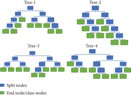
It is important to note that, out of the whole dataset, a certain amount of data vector is designated for training and rest which are kept for out-of-bag estimation. Once the model is trained, it can predict a new set of data with the majority vote of the trees. For any input data vector X, it can be defined as

()

where P(X)_z symbolizes the prediction of zth tree.

Furthermore, the limitation of RF is high variance and biasing that arises fitting issues. That means a delta amount of change in training data is supposed to create a completely different variant of decision trees. However, the problem of underfitting and overfitting is effectively addresses through two primary strategies: bagging and random feature selection. Bagging entails creating multiple subsets of the training data by sampling with replacement. Each subset undergoes training with a decision tree. This approach diminishes the model’s variance, reducing its sensitivity to noise or outliers in the data. Another important strategy is random feature selection, where instead of using all features at each split of the decision tree, a random subset of features is chosen. This helps minimize the correlation among trees and boosts the model’s resilience to irrelevant or redundant features. By combining these two techniques, the random decision forest achieves a well-balanced trade-off between bias and variance, effectively managing challenges related to underfitting and overfitting issues [41, 42].

3. Systems under Study

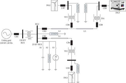
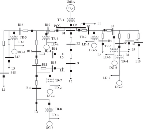
In this study, the validations are made with two separate test systems, namely, TS-I and TS-II, to ensure the dynamism of the proposed work. The first microgrid TS-I [40] is connected to a central grid at 120 kV bus which can be intentionally islanded by operating circuit breaker 1 (CB1). The related TS-I parameters are summarized in Table 1. The main transformer TF1 steps down the voltage from 120 kV to 25 kV and connected to the PCC at the low voltage end. Figure 2 shows the one-line diagram of TS-I that comprises of 3 DGs at separate location. On the other hand, the TS-II is consisting of 7 numbers of DGs where DG-1,2,7 are wind farms, DG-3,5,6 are diesel generators deployed in the time of emergency, and DG-4 is alone a PV unit. It is shown in Figure 3. The specifications of TS-II are presented in [43].

Table 1. Parameters of TS-I.

Parameters	Specification
Utility grid	120 kV, 60 Hz
DG1, DG2	9 MW wind system, 6 units of 1.5 MW, 60 Hz, 575 V
DG3	3.125 MVA synchronous diesel engine, 60 Hz, 575 V
Switching capacitor (C)	25 kV, 2 MVAR
Induction motor (M)	6 MVA
TF1	25 MVA, 120 kV/25 kV star-delta
TF2, TF3	12 MVA, 25 kV/575 V delta-star
TF4	5 MVA, 25 kV/575 V delta-star
L1, L2, L3	22 km, 60 Hz, 3-phase π-section line
LOAD3,4	8 MW, 1.75 MVAR
LD5	2.5 MW, 0.75 MVAR
LOAD1,2	6 MW, 1.4 MVAR

4. Data Collection and Feature Extraction

The purpose of the study is classification of disturbance events with machine learning which requires labelled dataset. Thus, dataset formation is very essential while implementing any MLC algorithm. But the preliminary step is to accumulate the skeletal parts of the dataset, i.e., features. This is done by the following steps:

(a)
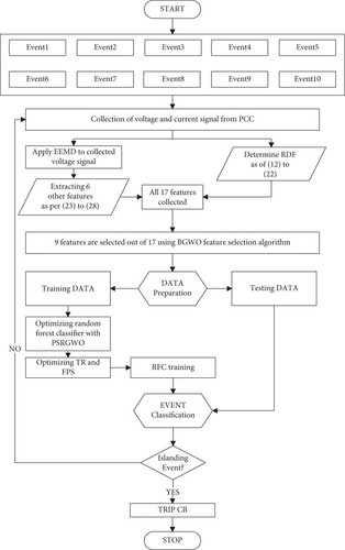
The voltage and current signals form the PCC are collected from few cycles and saved as time series data
(b)
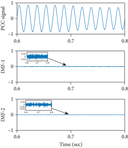
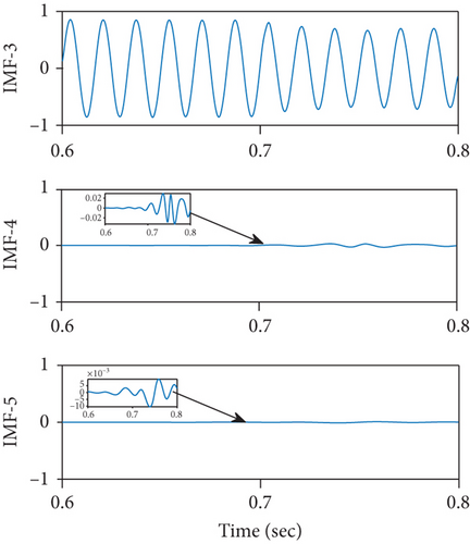
The signals are sampled uniformly at 2.4 kHz, and data samples are stored within a time frame of 0.6 to 0.8 seconds as disturbance is intentionally occurred within this interval. This can be seen in Figures 4(a) and 4(b)
(c)
From the retrieved signals, 2 types of features are extracted, namely, raw signal features (RSFs) and decomposed signal features (DSFs)

The mathematical formulations of RSF and DSF are mentioned from Eq. (10)–(26). Here, (10)–(20) are for RSF and rest are applied on 3rd IMF of voltage signal to obtain DSF. Now for any signal y(k) having K number of samples, the features are represented as follows:

()

where V_{n_RMS} and I_{n_RMS} are the nth harmonic voltage/current and

and

are the fundamental voltage/current.

5. Methodology

There are several events in power system such as transformer/capacitor switching, load/line switching, and operating of circuit breakers that are wrongly identified as islanding events by the traditional detection schemes. The working flow of the proposed techniques is undetected due to low power mismatching which should be avoided. A flow diagram of the proposed work is presented in Figure 5 for detection of islanding and nonislanding (I&NI) events correctly. Keeping in mind the actual grid scenarios, a wide range of I&NI events are deliberately simulated in MATLAB Simulink environment. In this process, 10 different classes of events are obtained as explained in Table 2. For each event occurrence, both voltage and current signals are collected from PCC. From the collected signal, a total of 17 features including RSF and DSF are extracted. As discussed before, RSFs are calculated directly from raw signal, but DSFs are extracted from the 3rd IMF of the EEMD decomposed voltage signal. The motive behind considering the 3rd IMF and discarding others is only because of the highest similarity of this with respect to the disturbance signal. This can be visualized by Pearson’s correlation coefficient (PERCC). PERCC serves as a gauge for the linear relationship between two signals. Its value ranges from -1 to 1. This coefficient indicates a perfect negative correlation at -1, no correlation at 0, and a perfect positive correlation at 1. It can be defined as

()

where X_μ and Y_μ are the mean and X_σ and Y_σ are the standard deviation of the respective signals.

Table 2. Class of events.

Event classes	Name of event	Description	Samples
EC-1	Islanding	CB1 opening	800
EC-2	Outage of DG	DG-1	800
EC-3	Outage of DG	DG-2	800
EC-4	Capacitor switching	S1 switching	800
EC-5	Line switching	CB3 opening	800
EC-6	Induction motor switching	S3 switching	800
EC-7	Load switching	S2 switching	800
EC-8	Fault	LG, LLG, LLL, LLLG	200
EC-9	Voltage sag	At target DG	800
EC-10	Voltage swell	At target DG	800

The PERCC of all the IMFs to that of the healthy signal is given in Table 3. It clearly displays that IMF-3 has the highest correlation of 0.9137 with the disturbance signal and hence chosen for DSF extraction. Thus, 800 data instances of each EC have been saved to the database. An 8000 × 17 feature vector has been extracted in this procedure and fed to a FST called binary grey wolf optimizer (BGWO) which will eliminate the redundant features and only hold 9 uncorrelated features. Those are V_rms, I_THD, MEAN(dv/dt), MEAN(d²i/dt²), MEAN(df/dt), MEAN(dP/dt), ENG_f, DEV_f, and SKW_f. The objective function of BGWO is taken as the overall accuracy error (OAE). It is defined as

()

where OA stands for overall accuracy.

Table 3. Correlation of IMFs with healthy signal.

IMF_i	IMF1	IMF2	IMF3	IMF4	IMF5
PERCC	0.0173	0.0392	0.9137	0.1733	0.0851

Next, the compressed dataset undergoes data preparation stage where the data is get divided into training and testing data to fed into RFC. But with the focus on improving the efficacy of this classifier, a hybrid optimization technique, namely, PSO with reformed-GWO (PSRGWO), has been proposed in this paper. This hybrid optimizer is basically going to optimize two parameters. The detailed information regarding the application of PSRGWO is presented in the next subsection.

5.1. Hybrid PSO and Reformed GWO Algorithm (PSRGWO)

In this section, a hybrid algorithm is suggested combining the traditional particle swarm optimization with a reformed version of grey wolf optimization so as to strengthen the exploration capabilities. Here, within a single iteration of main loop, there exist few iterations of PSO followed by a few iterations of GWO. At the end of every loop, the outcomes of PSO and GWO are compared to save the best value till that particular iteration. As a result, the modified GWO will ensure the reduction in probability of PSO to get trapped in local extrema. The workflow of the proposed algorithm is shown in Figure 6.

Furthermore, there are few modifications which are imposed to the conventional GWO algorithm to make the entire optimization process more efficient. In any population-based optimization technique, the agents will first get distributed among the entire search space to explore it and then exploit the collected knowledge to converge the solution to global extremum. Mathematically, if

(as of 3), then exploring is going on and it continues till half of the total GWO iterations and in the next half of iterations

that carry out the exploitation work. As higher exploration reduces the possibility of local stagnation, the iteration dedicated to exploration can be increased by modifying (3). It is defined as

()

This will devote more than two-thirds of the total iterations for exploration job, and the rest are committed to exploitation. Secondly, there is a mere possibility of the solution to get trapped other than the major three wolves called omega (ὼ) wolves. For this cause, the positions of omega wolves are also updated in GWO reformation. It can be represented as

()

Thirdly, even though it was said in conventional GWO that the wolves are following a specific hierarchy but while updating the position vector equation, all three major wolves are treated equally as shown in (4). Here, the updating equation is rewritten with a weighted valuation of wolves. Thus, the reformed updating equation is as follows:

()

Moreover, the cost function used in such type of problems is generally based upon accuracy index. But in this error minimization problem, Cohen’s kappa error is minimized to ensure an optimum number of trees and especially least number of FPS. This will guarantee the highest accuracy with lowest correlations between trees. The kappa index can be mathematically represented as

()

where PA is the probability of agreement and PA_C is the probability of agreement by chance. Now the objective function of the minimization problem can be defined as

()

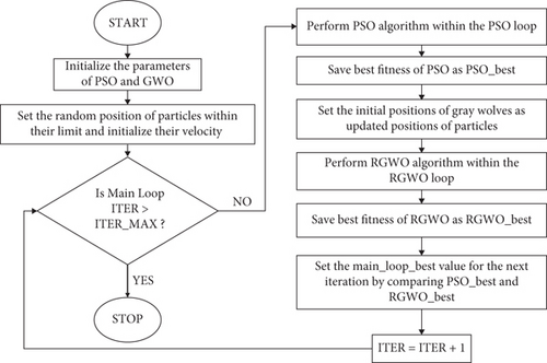
Here, ₭_error represents the kappa error, and ₭ represents the actual kappa index. These are function of number of trees (TR) in the forest and feature involved in each split (FPS) of any tree construction.

6. Result Analysis

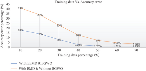
The proposed system is simulated in MATLAB (version 2018a) software running in a Lenovo personal computer with INTEL core-i5 8th generation 2.3 GHz processor and 8 GB RAM. The performance will be evaluated using the feature optimized dataset consisting of 9 distinct features (column wise) that holds 10 sets of event classes (row wise) to form an 8000 × 9 data vector. The collection of data samples is made under a wide range of power mismatch condition for both I&NI occurrences which results in a diversified dataset that have the seldom possibility of redundancy and biasing. Here, half of the data are taken for training and the remaining half for testing to verify the hybrid optimization-based random forest classifier (HOBRFC). Normally, a higher percentage of data (70 to 80%) are taken to train any classifier to ensure higher accuracy, but purity and clarity of data abstraction can play a vital role to amplify the performance indices of any classifier. A “training data percentage” versus “accuracy error” graph in Figure 7 can well describe the meaning of the previous statement. It can be observed that the reduced dataset can attain maximum prediction level even with 50% of training data. This signifies the unmatched data abstraction ability of EEMD as well as the unbiased feature selection capability of BGWO.

6.1. Optimal Parameter Selection for HOBRFC

RF classifier’s performance is based on the decision of several DTs whose branch division is carried out with a random subset of features. Training such type of models requires the dimensionality definition of both of these two elements which can be achieved using optimization. As we are optimizing TR and FPS, the preliminary requirement is to set the lower and upper limits of these two. The default FPS [42] in an RFC is chosen as , where p is the maximum number of available features. In this case, p = 9 so the lower limit of FPS is taken as 3. On the other side setting, the max value as the upper limit, certainly going against the core definition of the term “random” as this signifies any node of a DT inside the RF is subdivided into further branches using a random subset of features.

Moreover, a higher value of FPS can increase the correlation between the trees which in turn reduces their individuality. Hence, the upper limit of FPS is taken as 8 instead of 9. Further, setting the limits of TR is quite tricky. Choosing a much smaller lower limit can affect agreement to disagreement ratio as the decision-making of RF relies on collective voting approach. Since lower limit of FPS is 3 and maximum feature available is 9, a total of 84 combinations of feature subsets can be formed as per (33). If each subset is assumed to be used uniquely to split only a single node of a tree in the entire forest, it is required at least 9 trees to accommodate all. A glimpse of Figure 8 can well explain why it has been said. There are 4 example trees where blue-colored nodes are split nodes and green-colored nodes are end nodes or class nodes. It can be noted that, to reach 9 end nodes, there should be minimum 8 split nodes in a tree. As the end nodes of trees are the classes, at least “m − 1” node splits are needed to specify “m” classes in a tree. Since the number of classes is 10 over here and 9 node splits are required to make 10 end nodes, 84/10 = 8.4(≈9) trees are desired to accommodate 84 feature subsets. Hence, the lower limit of TR is set to be 9. Although RF never overfits while adding more and more numbers of trees [43], still it is important to find out the optimum trees for the classifier speed point of view. So, the upper limit can be decided by plotting, out-of-bag classification error (OBCE) vs. number of trees as shown in Figure 9. It can be seen that the OBCE remains stable approximately after 190 trees. Therefore, with a small margin, the upper limit is placed at 200.

()

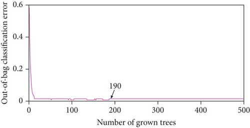
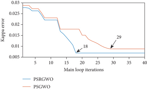
The parameters used during the implementation of proposed optimization algorithm are presented in Table 4. It can be seen from Figure 10 that PSRGWO’s performance is proving better both in terms of a number of iterations and error margin. While the PSGWO is taking 29 iterations to get the least converged error, on the other hand, the proposed PSRGWO is only taking 18 iterations to achieve an even low error margin. Finally, the optimum values of FPS (O_FPS) and TR (O_TR) are found to be 4 and 141, respectively, after taking the modes of 100 trails.

Table 4. Parameters of PSRGWO.

Parameters	Values	Parameters	Values
Max iteration of main loop	40	Search agents	20
Max iteration of PSO loop	15	Max iteration of GWO loop	15
Range of split features	[3 8]	Range of trees	[9 200]

6.2. Performance Indices

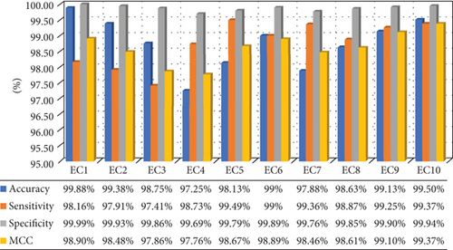
Performance indices (PIs) are the measures to analyze the prediction capability of a classifier once it is trained. It may sound a little weird if the formulae of different indices are directly stated over here. But it will be much easier to understand the PIs once after understanding the concept of the confusion matrix (CM). Simply, CM is a square matrix datasheet that estimates the performance of any ML classification model.

The core of the random forest machine learning model is decision trees, and each decision tree will train with random subset of features. Furthermore, the end nodes of these trees are the event classes. Therefore, a model trained with 10 classes will one islanding, and 9 PQ events (case 1) have separate tree structures than that of a model trained with only 9 PQ event classes (case 2). For this reason, the proposed model is tested with both the conditions.

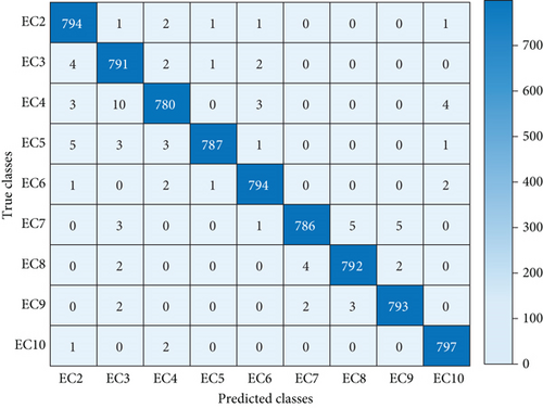
In Figure 11(a), the confusing matrix is obtained for the model trained with case 1, where 800 events per class are predicted using the proposed detection technique. It is found that the method shows 99.88% accuracy in detecting the islanding scenarios as 799 islanding cases are truly detected out of 800 classes. Apart from that, other nonislanding events are also showing promising accuracy of detection. Here, classes EC-1 to EC-10 are mapped as 1 to 10. Similarly, in Figure 11(b), only the case 2 events are considered. The proposed classifier also displays much accuracy for nonislanding events alone where EC-10 has highest accuracy rate of 99.63% since 797 events have predicted truly out of 800. Here, classes EC-2 to EC-10 are mapped as 1 to 9. The figures are represented as heatmaps. The darker color of the diagonal elements reflecting the elegant performance of the classifier. Now the above statement can be verified mathematically with the help of several PIs.

The mathematical formulae of several PIs such as accuracy, specificity, sensitivity, and Matthew’s correlation coefficient (MCC) are presented in the (35)–(38). Two bar chart distributions of all the PIs of every EC both under I&NI events are shown in Figures 12(a) and 12(b). Due to the randomness property of RF, all the indices are obtained by taking the mean of 100 trials. These results are ensuing the efficacy of the proposed HOBRFC which is well capable of detecting islanding and PQ disturbance events.

()

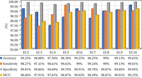
6.3. Noise Tolerance Evaluation

Noise is a nonavoidable part of any system, thus also visible in power system. The companionship of communication lines with power lines creates electromagnetic interference which is the main reason for noise existence in collected signal.

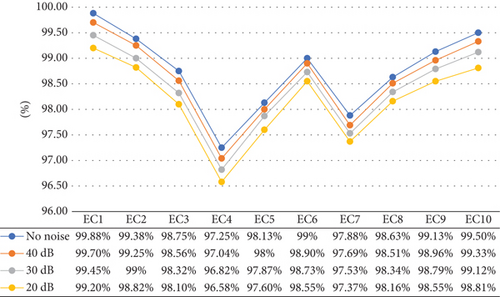
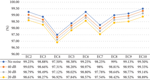
As the studied system is designed in MATLAB environment, to simulate the noisy condition, additive white Gaussian noise with 3 different signal-to-noise ratio is added to the collected signal. It can be expressed as

()

The proficiency of the suggested approach under noisy conditions can be contemplated in Figures 13(a) and 13(b). It is observed that the noise-free accuracy of important islanding events (EC-1) is reaching 99.88% whereas it is hitting 99.2% even under the dense noise of 20 dB. Similarly, the mean accuracies of the other events under islanding conditions represented by EC-2 to EC-10 are maintained at 98.79%, 98.58%, 98.39%, and 98.18% for 40 dB, 30 dB, and 20 dB SNR, respectively.

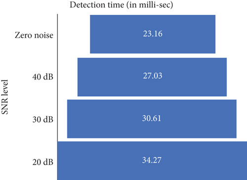
Additionally, the proposed EEMD-HOBRFC also provides faster detection of all the events, and it is noted to be only 23.16 msec under the ideal situation. The exceptional ability of the technique makes it to elapse almost same time to detect any type of trained event. But the performance is stagnated with the introduction of noise. A series of 500 disturbance cases is taken for each SNR level, and the mean time of detection is illustrated in Figure 14.

6.4. Performance Assessment in TS-II

The extraordinary efficacy of the EEMD-HOBRFC is already seen in the previous subsections for test system 1. However, it is essential to verify whether it is performing in the same manner or not for a different system. So as to validate it, a separate test system is taken into consideration as shown in Figure 3. A 400 number of cases are extracted for each event class only having the BGWO optimized prediction variables (9 numbers of features) from test system 2. This extraction has taken place in both islanding and nonislanding scenarios. The confusion matrix in relation to both the scenarios can be seen in Figures 15(a) and 15(b). It can be seen from Figure 15(a) that the method shows 100% accuracy in detecting the islanding scenarios as all the 400 cases are truly detected. Here, classes EC-1 to EC-10 are mapped as 1 to 10. On the other hand, the proposed classifier also displays much accuracy for nonislanding events alone where EC-15 has highest accuracy rate of 99.5% since 398 events have predicted truly out of 400. Here, classes EC-2 to EC-10 are mapped as 1 to 9.

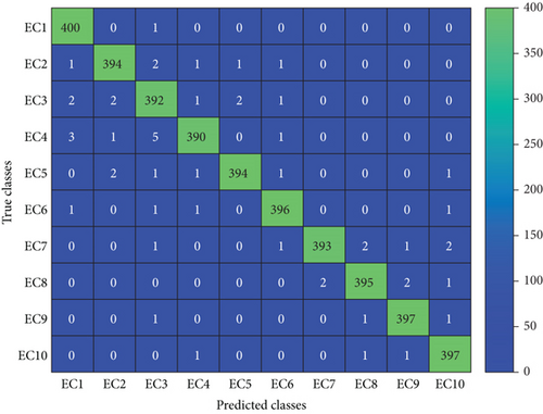
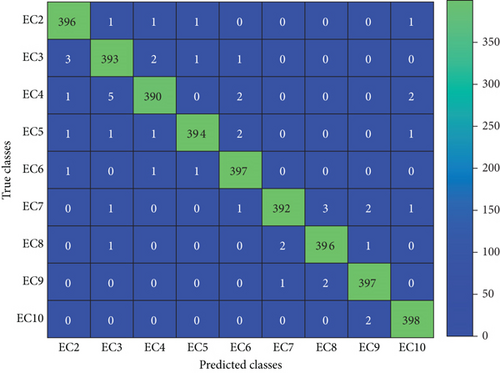
It can be noted that, under islanding condition (Figure 15(a)), the method of EEMD-HOBRFC successfully detected all the 400 islanding events. In addition, it is also displayed its detection capability for the other events with and without islanding occurrences. Hence, the proposed method is found to be effective even in other microgrid structures.

6.5. Comparative Study

This section covers up the comparative study of the proposed EEMD-HOBRFC method with several other methods. Firstly, both EMD and EEMD are combined with simple unoptimized RF and latterly clubbed with HOBRFC for 3 different SNR levels as presented in Table 5. The resulting accuracy data can well define the dominancy of the proposed method that reaching 99.2% under substantial noise (20 dB) and 99.88% without any noise. Moreover, Table 6 unveils its supremacy over other ML tools. It can be noticed that the EEMD-HOBRFC is displaying appreciable accuracy with respect to all these MLTs with maintaining a mean accuracy of 98.75%.

Table 5. Comparing with optimized and nonoptimized EMD and EEMD techniques.

Techniques	Zero noise	SNR level
Techniques	Zero noise	40 dB	30 dB	20 dB
EMD-RF	97.6%	97.4%	97.1%	96.6%
EMD-HOBRFC	98.6%	98.42%	98.24%	97.97%
EEMD-RF	99.1%	98.87%	98.69%	98.4%
EEMD-HOBRFC	99.88%	99.7%	99.45%	99.2%

Table 6. Comparing with other ML techniques with EEMD in absence of any noise.

Classes	NB	ELM	KNN	SVM	DT	Proposed
EC-1	93.58%	98.65%	98.81%	99.02%	99.3%	99.88%
EC-2	92.95%	98.11%	98.25%	98.47%	98.81%	99.38%
EC-3	92.78%	97.6%	97.77%	98.01%	98.33%	98.75%
EC-4	91%	96.07%	96.23%	96.43%	96.78%	97.25%
EC-5	91.72%	96.95%	97.09%	97.31%	97.6%	98.13%
EC-6	92.53%	97.76%	97.93%	98.15%	98.48%	99%
EC-7	91.47%	96.63%	96.8%	97.03%	97.34%	97.88%
EC-8	92.39%	97.5%	97.64%	97.87%	98.17%	98.63%
EC-9	92.75%	97.89%	98.03%	98.26%	98.61%	99.13%
EC-10	93.04%	98.18%	98.36%	98.55%	98.98%	99.50%
Mean	92.421%	97.534%	97.691%	97.91%	98.24%	98.75%

Further, the analysis is extended in terms of detection time, detection accuracy, and performance under noisy conditions. The time required for islanding detection for different preproposed techniques with their references can be seen in Table 7. The maximum detection time taken is around 55 ms for a transient monitoring [45] based detection system which is more than twice of the detection time of the proposed one. Besides that, the performance of the EEMD-HOBRFC is evaluated against other prepublished work in Table 7. Furthermore, in Table 8, it can be noticed that, although [48, 52] delivering an accuracy level of 100%, still they are underperforming in the presence of noise. But the proposed method has built up with both noise-assisted signal processing technique and noise robust machine learning technique that is why performing at towering level of accuracy in all three noisy conditions.

Table 7. Detection time of the proposed method with respect to other research works.

Sl no.	Related works ref.	Detection time
1	[6]	Less than 28 ms
2	[44]	45 to 60 ms
3	[45]	Less than 34 ms
4	[33]	40 ms
5	[46]	50 ms
6	[47]	Around 55 ms
7	Proposed	23.16 ms

Table 8. Accuracy tally with some of the prepublished articles.

Sl no.	Published work	Accuracy
Sl no.	Published work	Noise free	20 dB	30 dB	40 dB
1	[26]	98.8%	98.3%	97.5%	97%
2	[34]	99.09%	91.51%	96.96%	—
3	[48]	100%	97.66%	—	—
4	[49]	98.19%	—	—	—
5	[50]	98%	—	—	—
6	[51]	—	—	98.3%	—
7	[52]	100%	90%	98.78%	—
8	[53]	99.33%	—	—	—
9	[54]	98%	94.2%	—	—
10	Proposed	99.88%	99.2%	99.45%	99.7%

6.6. Nondetection Zone Validation

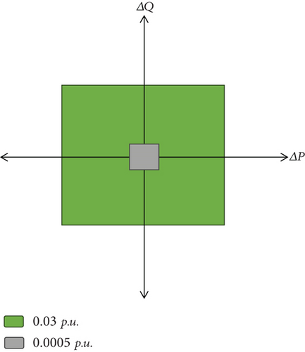
The contraction of NDZ can be validated by considering a mix of 500 diversified islanding data samples within a power mismatch range of 0.0005 pu to 0.03 pu with 30 dB SNR. Even in such a narrow range, the EEMD-HOBRFC is still capable of detecting 498 islanding event classes. The other two are detected falsely as DG outage and capacitor switching. The outcomes not only indicate the impact of the proposed method under low power mismatch conditions but also replicate the efficacy under the noisy situations. That means it can be well implemented in practical environment. The result of this test is given in Table 9, and the contracted region of nondetection is shown in grey color in Figure 16.

Table 9. Event detection inside narrow range to validate NDZ.

True class	Predicted class
True class	EC-1	EC-2	EC-3	EC-4	EC-5	EC-6	EC-7	EC-8	EC-9	EC-10
EC-1	498	1	0	1	0	0	0	0	0	0

7. Conclusion

The manuscript presents an islanding detection scheme, namely, EEMD-HOBRFC, that can identify and classify the islanding as well as nonislanding power quality events. In the proposed approach, some of the features are retrieved from the raw signal to retain the original characteristics of the signal and the rest of the features are extracted from the decomposition of noise-assisted signal preprocessor called EEMD to capture the inherent characteristics.

Moreover, the least correlated features are filtered with BGWO and then fed to a PSRGWO optimized random forest classifier. The proposed technique is validated with a system consisting of multi-DG system with high wind energy penetration, and accuracy of islanding detection under ideal condition is found to be 99.88%.

Its performance is not worsening under noisy condition and maintained at 99.2% even in the dense noise of 20 dB because both EEMD and RF are noise robust in nature. Additionally, the detection time is found to be as low as 23.16 ms with no noise and 34.27 ms at heavier noise.

Lastly, the method is also able to detect islanding event in real scenario (30 dB SNR) alongside a power mismatch range of 0.03 pu to 0.005 pu with an appreciable accuracy of 99.6%. Hence, the method is found to be very competitive with reference to the related research works of recent past. From rigorous simulation study, it is found that the proposed EEMD-HOBRFC is able to detect and classify the islanding and nonislanding event classes efficiently.

Abbreviations

BGWO:: Binary grey wolf optimization
CM:: Confusion matrix
DG:: Distributed generator
DSF:: Decomposed signal feature
DT:: Decision tree
EC:: Event class
EEMD:: Ensemble empirical mode decomposition
EMD:: Empirical mode decomposition
EWT:: Empirical wavelet transform
FPS:: Feature per split
FST:: Feature selection tool
GWO:: Grey wolf optimization
HOBRFC:: Hybrid optimization-based random forest classifier
I&NI:: Islanding and nonislanding
IMF:: Intrinsic mode function
MCC:: Matthew’s correlation coefficient
MLC:: Machine learning classifier
NDZ:: Nondetection zone
OAE:: Overall accuracy error
OBCE:: Out-of-bag classification error
PCC:: Point of common coupling
PERCC:: Pearson’s correlation coefficient
PI:: Performance index
PSRGWO:: Particle swarm and reformed grey wolf optimization
RF:: Random forest
RSF:: Raw signal feature
SPA:: Signal processing approach
TR:: Number of tress in forest
TS:: Test system
VMD:: Variational mode decomposition.

Conflicts of Interest

The authors declare that they have no conflicts of interest.

Acknowledgments

The authors extend their appreciation to the Deanship of Scientific Research at Northern Border University, Arar, KSA, for funding this research work through the project number NBU-FPEJ-2024-2484-01; also, the authors declare that this article has been produced with the financial support of the European Union under the REFRESH—Research Excellence For Region Sustainability and High-Tech Industries project number CZ.10.03.01/00/22_003/0000048 via the Operational Program Just Transition, and the paper was supported by the following project TN02000025 National Centre for Energy II.

Open Research

Data Availability

There are no data to mention.

References

1 Standards Board I. E. E. E., IEEE Standard for Interconnecting Distributed Resources with Electric Power Systems: 1547-2003, 2003, IEEE.
Google Scholar
2 Ropp M. E., Begovic M., and Rohatgi A., Analysis and performance assessment of the active frequency drift method of islanding prevention, IEEE Transactions on Energy Conversion. (1999) 14, no. 3, 810–816, https://doi.org/10.1109/60.790956, 2-s2.0-0033345608.
10.1109/60.790956
Web of Science® Google Scholar
3 Bower W. I. and Ropp M., Evaluation of islanding detection methods for utility-interactive inverters in photovoltaic systems (no. SAND2002-3591), 2002, Sandia National lab.(SNL-NM), Albuquerque, NM (United States); Sandia National Lab.(SNL-CA), Livermore, CA (United States).
10.2172/806700
Google Scholar
4 Freitas W., Xu W., Affonso C. M., and Huang Z., Comparative analysis between ROCOF and vector surge relays for distributed generation applications, IEEE Transactions on Power Delivery. (2005) 20, no. 2, 1315–1324, https://doi.org/10.1109/TPWRD.2004.834869, 2-s2.0-17744386563.
10.1109/TPWRD.2004.834869
Web of Science® Google Scholar
5 Liu S., Zhuang S., Xu Q., and Xiao J., Improved voltage shift islanding detection method for multi-inverter grid-connected photovoltaic systems, IET Generation, Transmission & Distribution. (2016) 10, no. 13, 3163–3169, https://doi.org/10.1049/iet-gtd.2015.1151, 2-s2.0-84990063413.
10.1049/iet-gtd.2015.1151
Web of Science® Google Scholar
6 Ray P. K., Mohanty S. R., and Kishor N., Disturbance detection in grid-connected distributed generation system using wavelet and S-transform, Electric Power Systems Research. (2011) 81, no. 3, 805–819, https://doi.org/10.1016/j.epsr.2010.11.011, 2-s2.0-78650937810.
10.1016/j.epsr.2010.11.011
Web of Science® Google Scholar
7 Raza S., Mokhlis H., Arof H., Laghari J. A., and Wang L., Application of signal processing techniques for islanding detection of distributed generation in distribution network: a review, Energy Conversion and Management. (2015) 96, 613–624, https://doi.org/10.1016/j.enconman.2015.03.029, 2-s2.0-84925611901.
10.1016/j.enconman.2015.03.029
Web of Science® Google Scholar
8 Huang N. E., Shen Z., Long S. R., Wu M. C., Shih H. H., Zheng Q., and Liu H. H., The empirical mode decomposition and the Hilbert spectrum for nonlinear and non-stationary time series analysis. Proceedings of the Royal Society of London, Series A: Mathematical, Physical and Engineering Sciences. (1998) 454, no. 1971, 903–995.
10.1098/rspa.1998.0193
Web of Science® Google Scholar
9 Admasie S., Bukhari S. B. A., Bengovik Haider R., Gush T., and Kim C. H., A passive islanding detection scheme using variational mode decomposition-based mode singular entropy for integrated microgrids, Electric Power Systems Research. (2019) 177, article 105983, https://doi.org/10.1016/j.epsr.2019.105983, 2-s2.0-85070916198.
10.1016/j.epsr.2019.105983
Web of Science® Google Scholar
10 Gilles J., Empirical wavelet transform, IEEE Transactions on Signal Processing. (2013) 61, no. 16, 3999–4010, https://doi.org/10.1109/TSP.2013.2265222, 2-s2.0-84880891329.
10.1109/TSP.2013.2265222
Web of Science® Google Scholar
11 Wu Z. and Huang N. E., Ensemble empirical mode decomposition: a noise-assisted data analysis method, Advances in Adaptive Data Analysis. (2009) 1, no. 1, 1–41, https://doi.org/10.1142/S1793536909000047, 2-s2.0-80052078099.
10.1142/S1793536909000047
Google Scholar
12 Anand A. and Affijulla S., Ensemble empirical mode decomposition-based differential protection scheme for islanded and grid-tied AC microgrid, IET Generation, Transmission & Distribution. (2020) 14, no. 26, 6674–6681, https://doi.org/10.1049/iet-gtd.2020.1117.
10.1049/iet-gtd.2020.1117
Web of Science® Google Scholar
13 Zhang Z. and Hong W. C., Electric load forecasting by complete ensemble empirical mode decomposition adaptive noise and support vector regression with quantum-based dragonfly algorithm, Nonlinear Dynamics. (2019) 98, no. 2, 1107–1136, https://doi.org/10.1007/s11071-019-05252-7, 2-s2.0-85073688051.
10.1007/s11071-019-05252-7
Web of Science® Google Scholar
14 Santhosh M., Venkaiah C., and Kumar D. V., Ensemble empirical mode decomposition based adaptive wavelet neural network method for wind speed prediction, Energy Conversion and Management. (2018) 168, 482–493, https://doi.org/10.1016/j.enconman.2018.04.099, 2-s2.0-85046718866.
10.1016/j.enconman.2018.04.099
Web of Science® Google Scholar
15 Laghari J. A., Mokhlis H., Karimi M., Bakar A. H. A., and Mohamad H., Computational intelligence based techniques for islanding detection of distributed generation in distribution network: a review, Energy Conversion and Management. (2014) 88, 139–152, https://doi.org/10.1016/j.enconman.2014.08.024, 2-s2.0-84907483554.
10.1016/j.enconman.2014.08.024
Web of Science® Google Scholar
16 Duda R. O. and Hart P. E., Pattern classification, 2006, John Wiley & Sons.
Google Scholar
17 Dashtdar M., Flah A., Hosseinimoghadam S. M. S., Rami Reddy C., Kotb H., AboRas K. M., and Bortoni E. C., Improving the power quality of island microgrid with voltage and frequency control based on a hybrid genetic algorithm and PSO, IEEE Access. (2022) 10, 105352–105365, https://doi.org/10.1109/ACCESS.2022.3201819.
10.1109/ACCESS.2022.3201819
Web of Science® Google Scholar
18 Vashishtha G., Chauhan S., Kumar A., and Kumar R., An ameliorated African vulture optimization algorithm to diagnose the rolling bearing defects, Measurement Science and Technology. (2022) 33, no. 7, article 075013, https://doi.org/10.1088/1361-6501/ac656a.
10.1088/1361-6501/ac656a
PubMed Web of Science® Google Scholar
19 Dashtdar M., Flah A., Hosseinimoghadam S. M. S., Kotb H., Jasińska E., Gono R., Leonowicz Z., and Jasiński M., Optimal operation of microgrids with demand-side management based on a combination of genetic algorithm and artificial bee colony, Sustainability. (2022) 14, no. 11, https://doi.org/10.3390/su14116759.
10.3390/su14116759
Web of Science® Google Scholar
20 Babanezhad M., Arabi Nowdeh S., Abdelaziz A. Y., AboRas K. M., and Kotb H., Reactive power based capacitors allocation in distribution network using mathematical remora optimization algorithm considering operation cost and loading conditions, Alexandria Engineering Journal. (2022) 61, no. 12, 10511–10526, https://doi.org/10.1016/j.aej.2022.04.009.
10.1016/j.aej.2022.04.009
Web of Science® Google Scholar
21 Rashedi E., Nezamabadi-Pour H., and Saryazdi S., BGSA: binary gravitational search algorithm, Natural Computing. (2010) 9, no. 3, 727–745, https://doi.org/10.1007/s11047-009-9175-3, 2-s2.0-77955923868.
10.1007/s11047-009-9175-3
Web of Science® Google Scholar
22 Nakamura R. Y., Pereira L. A., Costa K. A., Rodrigues D., Papa J. P., and Yang X. S., BBA: a binary bat algorithm for feature selection, 2012 25th SIBGRAPI Conference on Graphics, Patterns and Images, 2012, Ouro Preto, Brazil, https://doi.org/10.1109/SIBGRAPI.2012.47, 2-s2.0-84872367831.
10.1109/SIBGRAPI.2012.47
Google Scholar
23 Emary E., Zawbaa H. M., and Hassanien A. E., Binary ant lion approaches for feature selection, Neurocomputing. (2016) 213, 54–65, https://doi.org/10.1016/j.neucom.2016.03.101, 2-s2.0-84994810199.
10.1016/j.neucom.2016.03.101
Web of Science® Google Scholar
24 Vashishtha G. and Kumar R., An amended grey wolf optimization with mutation strategy to diagnose bucket defects in Pelton wheel, Measurement. (2022) 187, article 110272, https://doi.org/10.1016/j.measurement.2021.110272.
10.1016/j.measurement.2021.110272
Web of Science® Google Scholar
25 Emary E., Zawbaa H. M., and Hassanien A. E., Binary grey wolf optimization approaches for feature selection, Neurocomputing. (2016) 172, 371–381, https://doi.org/10.1016/j.neucom.2015.06.083, 2-s2.0-84946490956.
10.1016/j.neucom.2015.06.083
Web of Science® Google Scholar
26 Ahmadipour M., Hizam H., Lutfi Othman M., and Amran Mohd Radzi M., An anti-islanding protection technique using a wavelet packet transform and a probabilistic neural network, Energies. (2018) 11, no. 10, https://doi.org/10.3390/en11102701, 2-s2.0-85056144261.
10.3390/en11102701
Web of Science® Google Scholar
27 Jasim A. M., Jasim B. H., Aymen F., Kotb H., and Althobaiti A., Consensus-based intelligent distributed secondary control for multiagent islanded microgrid, International Transactions on Electrical Energy Systems. (2023) 2023, article 6812351, 1–20, https://doi.org/10.1155/2023/6812351.
10.1155/2023/6812351
Web of Science® Google Scholar
28 Korkmaz M. E., Gupta M. K., Kuntoğlu M., Patange A. D., Ross N. S., Yılmaz H., Chauhan S., and Vashishtha G., Prediction and classification of tool wear and its state in sustainable machining of Bohler steel with different machine learning models, Measurement. (2023) 223, article 113825, https://doi.org/10.1016/j.measurement.2023.113825.
10.1016/j.measurement.2023.113825
Web of Science® Google Scholar
29 Vashishtha G. and Kumar R., Unsupervised learning model of sparse filtering enhanced using Wasserstein distance for intelligent fault diagnosis, Journal of Vibration Engineering & Technologies. (2023) 11, no. 7, 2985–3002, https://doi.org/10.1007/s42417-022-00725-3.
10.1007/s42417-022-00725-3
Web of Science® Google Scholar
30 Vashishtha G., Chauhan S., Yadav N., Kumar A., and Kumar R., A two-level adaptive chirp mode decomposition and tangent entropy in estimation of single-valued neutrosophic cross-entropy for detecting impeller defects in centrifugal pump, Applied Acoustics. (2022) 197, article 108905, https://doi.org/10.1016/j.apacoust.2022.108905.
10.1016/j.apacoust.2022.108905
Web of Science® Google Scholar
31 Shahryari E., Nooshyar M., and Sobhani B., Combination of neural network and wavelet transform for islanding detection of distributed generation in a small-scale network, International Journal of Ambient Energy. (2019) 40, no. 3, 263–273, https://doi.org/10.1080/01430750.2017.1392348, 2-s2.0-85032366125.
10.1080/01430750.2017.1392348
CAS Web of Science® Google Scholar
32 Gomes E. A., Vieira J. C., Coury D. V., and Delbem A. C., Islanding detection of synchronous distributed generators using data mining complex correlations, IET Generation, Transmission & Distribution. (2018) 12, no. 17, 3935–3942, https://doi.org/10.1049/iet-gtd.2017.1722, 2-s2.0-85053605177.
10.1049/iet-gtd.2017.1722
Web of Science® Google Scholar
33 Mlakić D., Baghaee H. R., and Nikolovski S., A novel ANFIS-based islanding detection for inverter-interfaced microgrids, IEEE Transactions on Smart Grid. (2019) 10, no. 4, 4411–4424, https://doi.org/10.1109/TSG.2018.2859360, 2-s2.0-85050611845.
10.1109/TSG.2018.2859360
Web of Science® Google Scholar
34 Mishra M., Sahani M., and Rout P. K., An islanding detection algorithm for distributed generation based on Hilbert–Huang transform and extreme learning machine, Sustainable Energy, Grids and Networks. (2017) 9, 13–26, https://doi.org/10.1016/j.segan.2016.11.002, 2-s2.0-84998829028.
10.1016/j.segan.2016.11.002
Web of Science® Google Scholar
35 Ali J., Khan R., Ahmad N., and Maqsood I., Random forests and decision trees, International Journal of Computer Science Issues (IJCSI). (2012) 9, no. 5.
Google Scholar
36 Fernández-Delgado M., Cernadas E., Barro S., and Amorim D., Do we need hundreds of classifiers to solve real world classification problems?, The Journal of Machine Learning Research. (2014) 15, no. 1, 3133–3181.
Web of Science® Google Scholar
37 Ben-David A., Comparison of classification accuracy using Cohen’s weighted kappa, Expert Systems with Applications. (2008) 34, no. 2, 825–832, https://doi.org/10.1016/j.eswa.2006.10.022, 2-s2.0-36148976852.
10.1016/j.eswa.2006.10.022
Web of Science® Google Scholar
38 Vieira S. M., Kaymak U., and Sousa J. M., Cohen′s kappa coefficient as a performance measure for feature selection, International Conference on Fuzzy Systems, 2010, Barcelona, Spain, https://doi.org/10.1109/FUZZY.2010.5584447, 2-s2.0-78549269455.
10.1109/FUZZY.2010.5584447
Google Scholar
39 Ray P. K., Kishor N., and Mohanty S. R., Islanding and power quality disturbance detection in grid-connected hybrid power system using wavelet and $ S $-transform, IEEE Transactions on Smart Grid. (2012) 3, no. 3, 1082–1094, https://doi.org/10.1109/TSG.2012.2197642, 2-s2.0-84865515696.
10.1109/TSG.2012.2197642
Web of Science® Google Scholar
40 Farhan M. A. and Shanti Swarup K., Mathematical morphology-based islanding detection for distributed generation, IET Generation, Transmission & Distribution. (2016) 10, no. 2, 518–525, https://doi.org/10.1049/iet-gtd.2015.0910, 2-s2.0-84958793829.
10.1049/iet-gtd.2015.0910
Web of Science® Google Scholar
41 Azar A. T., Elshazly H. I., Hassanien A. E., and Elkorany A. M., A random forest classifier for lymph diseases, Computer Methods and Programs in Biomedicine. (2014) 113, no. 2, 465–473, https://doi.org/10.1016/j.cmpb.2013.11.004, 2-s2.0-84892819576.
10.1016/j.cmpb.2013.11.004
PubMed Web of Science® Google Scholar
42 Zhang C., Li Y., Yu Z., and Tian F., Feature selection of power system transient stability assessment based on random forest and recursive feature elimination, 2016 IEEE PES Asia-Pacific Power and Energy Engineering Conference (APPEEC), 2016, Xi’an, China, 1264–1268, https://doi.org/10.1109/APPEEC.2016.7779696, 2-s2.0-85010002100.
10.1109/APPEEC.2016.7779696
Google Scholar
43 Samui A. and Samantaray S. R., Wavelet singular entropy-based islanding detection in distributed generation, IEEE Transactions on Power Delivery. (2013) 28, no. 1, 411–418, https://doi.org/10.1109/TPWRD.2012.2220987, 2-s2.0-84871719683.
10.1109/TPWRD.2012.2220987
Web of Science® Google Scholar
44 Baghaee H. R., Mlakić D., Nikolovski S., and Dragicčvić T., Anti-islanding protection of PV-based microgrids consisting of PHEVs using SVMs, IEEE Transactions on Smart Grid. (2020) 11, no. 1, 483–500, https://doi.org/10.1109/TSG.2019.2924290.
10.1109/TSG.2019.2924290
Web of Science® Google Scholar
45 Niaki A. M. and Afsharnia S., A new passive islanding detection method and its performance evaluation for multi-DG systems, Electric Power Systems Research. (2014) 110, 180–187, https://doi.org/10.1016/j.epsr.2014.01.016, 2-s2.0-84894384257.
10.1016/j.epsr.2014.01.016
Web of Science® Google Scholar
46 Matic-Cuka B. and Kezunovic M., Islanding detection for inverter-based distributed generation using support vector machine method, IEEE Transactions on Smart Grid. (2014) 5, no. 6, 2676–2686, https://doi.org/10.1109/TSG.2014.2338736, 2-s2.0-84908303686.
10.1109/TSG.2014.2338736
Web of Science® Google Scholar
47 Dubey R., Popov M., and Samantaray S. R., Transient monitoring function-based islanding detection in power distribution network, IET Generation, Transmission & Distribution. (2019) 13, no. 6, 805–813, https://doi.org/10.1049/iet-gtd.2017.1941, 2-s2.0-85065121530.
10.1049/iet-gtd.2017.1941
Web of Science® Google Scholar
48 Ahmadipour M., Hizam H., Othman M. L., Radzi M. A. M., and Murthy A. S., Islanding detection technique using slantlet transform and ridgelet probabilistic neural network in grid-connected photovoltaic system, Applied Energy. (2018) 231, 645–659, https://doi.org/10.1016/j.apenergy.2018.09.145, 2-s2.0-85053805780.
10.1016/j.apenergy.2018.09.145
Web of Science® Google Scholar
49 Moeini A., Darabi A., Rafiei S. M. R., and Karimi M., Intelligent islanding detection of a synchronous distributed generation using governor signal clustering, Electric Power Systems Research. (2011) 81, no. 2, 608–616, https://doi.org/10.1016/j.epsr.2010.10.023, 2-s2.0-78650614353.
10.1016/j.epsr.2010.10.023
Web of Science® Google Scholar
50 Faqhruldin O. N., El-Saadany E. F., and Zeineldin H. H., A universal islanding detection technique for distributed generation using pattern recognition, IEEE Transactions on Smart Grid. (2014) 5, no. 4, 1985–1992, https://doi.org/10.1109/TSG.2014.2302439, 2-s2.0-84903219032.
10.1109/TSG.2014.2302439
Web of Science® Google Scholar
51 Kong X., Xu X., Yan Z., Chen S., Yang H., and Han D., Deep learning hybrid method for islanding detection in distributed generation, Applied Energy. (2018) 210, 776–785, https://doi.org/10.1016/j.apenergy.2017.08.014, 2-s2.0-85028310474.
10.1016/j.apenergy.2017.08.014
Web of Science® Google Scholar
52 Mishra M. and Rout P. K., Fast discrete s-transform and extreme learning machine based approach to islanding detection in grid-connected distributed generation, Energy Systems. (2019) 10, no. 3, 757–789, https://doi.org/10.1007/s12667-018-0285-9, 2-s2.0-85052399811.
10.1007/s12667-018-0285-9
Google Scholar
53 Alam M. R., Begum M. T. A., and Mather B., Islanding detection of distributed generation using electrical variables in space vector domain, IEEE Transactions on Power Delivery. (2020) 35, no. 2, 861–870, https://doi.org/10.1109/TPWRD.2019.2929784.
10.1109/TPWRD.2019.2929784
Web of Science® Google Scholar
54 Kumar S. A., Subathra M. S. P., Kumar N. M., Malvoni M., Sairamya N. J., George S. T., Suviseshamuthu E. S., and Chopra S. S., A novel islanding detection technique for a resilient photovoltaic-based distributed power generation system using a tunable-q wavelet transform and an artificial neural network, Energies. (2020) 13, no. 16, https://doi.org/10.3390/en13164238.
10.3390/en13164238
Web of Science® Google Scholar

Citing Literature

All articles

Islanding Detection and Power Quality Diagnosis of Wind Power Integrated Microgrid with Reduced Feature Trained Novel Optimized Random Decision Forest

Abstract

1. Introduction