1. Introduction

The detection of structural damage is an essential activity in assessing the life extension and safety of a structure during its service life [1, 2]. The essence of structural damage identification is an inverse problem in which the current data of a structure are used to evaluate the structural state and, thus, achieve the goal of assessing structural damage. This goal can be achieved in two ways: (1) pattern recognition and (2) solving a series of inverse problems [3, 4]. Civera et al. [5] introduced a fast relaxed vector fitting (FRVF) method for system identification in structural health monitoring, which demonstrated improvements in nonlinear fitting and robustness to noise compared to traditional methods. Xu et al. [6] investigated a structural damage identification method based on limited modal measurements and ultra-sparse Bayesian regression, which solved the problem of incomplete modal measurements by the ultra-sparse estimator. Boscato et al. [7] presented a regression method called Tree Gaussian Process (TGP) for assessing the structural condition of complex structural materials. The efficacy of TGP was verified on simply supported beams and two-dimensional frame structures. Figueiredo and Brownjohn [8] summarized the research and application of statistical pattern recognition methods in bridge health monitoring over the last three decades, including developments in sensing technology and data analysis. Dessena et al. [9] verified the effectiveness of the Loewner framework (LF) method for extracting modal parameters in structural health monitoring. Numerical modelling and experiments showed that LF can accurately identify modal parameters and find the differences between different damage states.

The inverse matrix plays a critical role in solving these inverse problems for static and dynamic damage identification. For static damage identification, Sanayei et al. [10–12] transformed damage identification into a linear-parameter estimation problem and performed analyses to achieve damage identification of elements using static data, of which inversion of the parameterized stiffness matrix is a crucial step. Viola and Bocchini [13] introduced a damage detection method for the systematic identification of nondestructive parameters in truss structures by static testing. The effectiveness of the proposed method was verified using several numerical models. Xiao et al. [14] obtained the displacements of truss and frame structures by inverting the stiffness matrix, which was transformed into an optimization problem for damage identification. For dynamic damage identification, Ren and De Roeck [15] proposed a technique for damage identification based on the variations in the vibration frequency and vibration pattern by multiplying the damaged eigenvalue equation with the damaged or undamaged mode to obtain more equations. Finally, the equations were solved for damage localization. Hwang and Kim [16] developed a damage detection method that used a frequency-response function to identify the location and severity of damage in a structure. The unknown stiffness parameters were identified as variables, and the frequency-response function matrix of the measured structure was inversely calculated, which, in turn, determined the location and degree of damage to the structure. Katebi et al. [17] used the inverses of the stiffness and flexibility matrices to identify damage and implemented static and dynamic deflections in parallel.

However, the inversion of the entire matrix becomes challenging as the size and complexity of the structure increases over time, and the structural freedom increases correspondingly. First, increasing the size of the matrix increases the storage and computation time. The complexity of matrix computation is often directly related to the dimensionality of the matrix [18–20]. Second, large structures contain more unknowns in damage detection, which can increase computational costs and cause possible ill-conditioning [21, 22]. Third, structural damage often occurs at local positions where the stiffness matrix varies sparsely, and the matrix inversion is always full, and it is uneconomical to invert the sparse matrix as a whole [23]. Researchers in many fields seek to improve matrix inversion efficiency while reducing the computational cost [24]. Therefore, scholars have proposed various solutions to this problem. With the advancement of mathematical and computational techniques, methods have been developed to improve the efficiency of matrix inverters in engineering. One class of methods improves the inversion efficiency primarily using algorithms. Rezaiee-Pajand and Kazemiyan [25] used four inversion methods to identify static damage to truss structures and compared their identification efficiencies. Boumechra [26] proposed the damage identification as an indicator of the corresponding static displacement under a moving load. Because of the complexity of the inverse matrix solution with corrective coefficients, they performed a Neumann decomposition of the stiffness formula. Qiao et al. [27] developed a group-sparse regularization method to identify the impact forces in the time domain. The group-sparse regularization method can efficiently and accurately identify continuous impact forces with massive dimensions and solve the inverse indeterminacy problem. Li et al. [28] proposed a method for locating structural acoustic emission sources based on the sparse decomposition of the near-field frequency space. This method reduces the sparsity of the matrix to reconstruct the signal using ergodic inversion, thus improving the computational efficiency of matrix inversion. Alebrahim et al. [29] used an improved QR decomposition-based method in which the sparsity of the matrices was considered. This method can compute the inverse of the stiffness matrix significantly faster than the traditional singular-value decomposition. Another class of methods starts from the main contradiction that larger matrices lead to inefficient inversion computations and uses dimensionality reduction to solve the matrix inverse problem. Huang et al. [30] used a block diagonal to solve an inverse with an excessively large dimension. Compared with solving the inverse directly, the computational complexity is significantly reduced. Feyzollahza and Bamdad [31] developed a matrix transposition method to solve the vibration of a rotating beam. This method significantly increases the matrix inversion efficiency and decreases the computation time by reducing the matrix order through adjustments of the carry-over zeros and matrix chunking. The application of the transfer matrix method to beam-like systems was subsequently investigated by their team [32]. In addition, some researchers combined the first two approaches to improve the matrix inversion efficiency. Xuebin et al. [33] proposed a modified in-place inversion algorithm to address the problem of long computation times attributed to medium-to-large inversion operations. This algorithm used a more sophisticated parallelization scheme to invert many small matrices on a CUDA platform. Zhou et al. [34] designed a graphic processing unit-based inversion algorithm that solved multiple forward and backward substitution subtasks in batches with improved results in terms of parallelism and convergence performance.

Although several algorithms have been developed to improve matrix efficiency, matrix inversion via a direct solution is still the main operation in engineering [35]. Based on previous studies, dimensionality reduction methods decrease computational complexity by reducing the matrix dimensionality, and the direct solution method is still used for low-dimensional matrices, which can prevent performance degradation [36]. In this study, the damage identification problem of a large-scale three-dimensional (3D) truss structure was investigated, and a stiffness separation method [37, 38] was applied to identify the damage to a truss structure. This method inverts only a part of the required stiffness matrix, reducing the number of matrix dimensions to be inverted. Thus, it can relatively solve the time-consuming calculation problem and improve the inversion efficiency. The two main objectives of this study are to refine the formulation of the stiffness separation method that considers the compatibility of displacements, external forces, and stiffness matrices and to demonstrate the effectiveness of the method by performing damage identification of a large truss structure under different damage conditions. Next, the size and region of the delineated substructure were changed to analyze the stiffness matrix dimensions and the effect of unknown parameters on matrix inversion and optimization.

2. Static Damage Identification Formula

This section presents the formulas for the space truss structure damage identification using a static response. The reduction in the cross-sectional area of the truss elements leads to decreased stiffness of the elements because the stiffness loss of structural elements is one of the main indicators of structural damage [39, 40]. Therefore, a reduction in the cross-sectional area of some truss elements was adopted in this study to indicate that damage had occurred to the structure. Suppose that $$ is the damaged member’s cross-sectional area, their values are unknown and included in the vector A_d. The following section presents a direct damage identification and stiffness separation method for analyzing space truss structures.

2.1. Direct Damage Identification Method

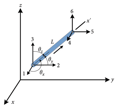
For a space truss member shown in Figure 1, the stiffness matrix of the truss element member in a local coordinate system is k^′.

The direction cosines between the global and local coordinates are defined as follows:

$$ ()

The displacement transformation matrix, T, transforms the displacements from member coordinates to global coordinates.

$$ ()

The member stiffness matrix expressed in global coordinates is k = T^Tk^′T. Consequently, for a general space truss structure, the entire structure’s global stiffness matrix K can be achieved by assembling k. Under the action of the global force component, Q, the global displacement is denoted as D, and the structural stiffness equation is Q = KD. The obtained structural stiffness matrix is blocked as follows to facilitate the calculations:

$$ ()

where Q_k and D_k are the known external forces and displacements, respectively, and Q_u and D_u are the unknown external forces and displacements, respectively. The division of the structural stiffness matrix must be compatible with the divisions of Q and D. However, because the cross-sectional area of the damaged members is unknown, the structural stiffness matrix contains unknown parameters of the damaged truss structure. For a damaged truss structure with known external loads and constraints, unknown displacements can be obtained using the following equation:

$$ ()

The analytical strain is then determined from the global displacement. The element strains of selected truss members are measured to identify the damage to the truss structure. In this study, the damage identification problem was transformed into a mathematical optimization problem, and optimization analysis was performed using a Nelder–Mead (NM) simplex algorithm to identify the parameters of the damaged members. The NM simplex algorithm is a direct search algorithm that seeks optimal values by comparing function values during the optimization process [41]. The objective function was set to the minimum value of the sum of squares of the measured and analyzed strain differences:

$$ ()

where ε_i is the measured strain of the member, s_i is the analytical strain of the member, and m is the total number of strain measurement points. The optimal cross-sectional area $$ of the damaged elements was obtained by optimizing the objective function.

$$ ()

3. Damage Identification of Space Truss Structure

In this part, the direct damage identification and stiffness separation method are applied to a space truss structure. The separated region was gradually reduced to analyze the impact on the computational efficiency of damage identification, and its number was varied to divide the damage to different substructures.

Figure 2 shows the space truss structure. The total length of the truss structure was 42 m, all the members had an original cross-sectional area of 3000 mm², and the modulus of elasticity was 206 GPa. In this study, the structure’s length, width, and height directions are designated as the X, Y, and Z directions, respectively. The positive axes X and Z are directed right and upward, respectively. The positive axis Y is directed from point 2 to 1 (Figure 2).

All the connections between the elements were pin-connected joints. The node and member numbers are shown in Figure 2. Nodes 1 and 2 are hinge supports, and Nodes 29 and 30 are roller supports. In addition, Nodes 4 and 27 were constrained to ensure the stability of the structure in the Y-direction.

Four damage conditions and several separate scenarios were investigated in this study. The damage conditions were divided into two parts: single-region and multi-region damage identification, and the unknown damage percentages for the members are between 5% and 40%.

3.1. Single-Region Damage Identification

In this section, two cases of truss damage are reported, where the damage occurs in one region. The stiffness separation method was used to separate the damage in a single region and conduct substructure damage identification.

Figure 3 shows damage condition A, which contains six damaged members in the left region of the structure. Members 2, 9, 12, 14, 17, and 18 are damaged, and their cross-sectional areas of damage condition A are listed in Table 1. In this study, strain sensors were located on the damaged members to obtain the measured strains.

Table 1. “As-is” cross-sectional areas of damage condition A.

Damaged member	Cross-sectional area $$ (mm2)
2	2850
9	2550
12	2700
14	2250
17	2400
18	2100

First, Figure 3(a) shows case 1, in which the damage to the entire structure is identified. External forces (10 kN) were applied to Nodes 13, 14, 17, and 18 to excite the entire structure. External forces (10 kN) were applied to Nodes 13 and 17 in the X- and negative Z-directions, and at Nodes 14 and 18 in the X-, negative Y-, and negative Z-directions.

Next, Figures 3(b), 3(c), 3(d), 3(e), and 3(f) show case 1-1 to case 1-5, in which displacement sensors were used to separate the substructure. In Figures 3(b), 3(c), 3(d), 3(e), and 3(f), the blue region of the structure represents the separated substructure, the red rectangles represent the strain sensor locations, and the red circles represent the displacement sensor locations, which are also the boundary nodes of the substructure. The DOFs of the separated regions decreased with changes in the location of the displacement sensor. For cases 1-1 to 1-5, loads were applied to Nodes 5 and 6 to receive a more pronounced static response in the damaged region. External forces (10 kN) were applied at Node 5 in the X- and negative Z-directions and at Node 6 in the X-, negative Y-, and negative Z-directions.

The damage in case 1 could be identified using the direct damage identification method, and cases 1-1 to 1-5 require the application of the stiffness separation method to separate the stiffness matrix and conduct the substructure damage identification. The key point is that equation (4) involves stiffness matrix inversion for damage identification, which is time-consuming for large-scale structures. This study aimed to reveal the relationship between the stiffness matrix dimension and matrix inversion time.

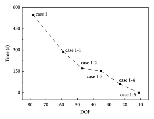
Table 2 records the inversion times for all the cases under damage condition A. Figure 4 shows a comparison of the inversion times for the different separation cases of damage condition A. In Figure 4, the horizontal axis represents the total number of unknown displacement DOFs in the substructure, and the corresponding DOFs for cases 1 and 1-1 to 1-5 are 78, 59, 47, 35, 23, and 11, respectively. The vertical axis represents the inversion time. In damage condition A, for a constant number of unknown parameters, the inversion time decreases as the unknown displacement DOFs of the substructure decrease.

Table 2. Inversion times of damage condition A.

Case	Case 1	Case 1-1	Case 1-2	Case 1-3	Case 1-4	Case 1-5
Time (s)	547.37	287.80	171.25	151.77	60.84	0.01

Next, the damage was identified for all cases of damage condition A based on equation (6). The mean relative error (MRE) is a statistical indicator used to determine the error between the identified and “as-is” values. The variation in the MRE during the identification process indicates the accuracy of the identification results. The MRE can be expressed as follows:

$$ ()

In equation (17), n is the total number of damaged members, $$ represents the optimized cross-sectional area of the d_i-th member in the entire structure, and $$ is the “as-is” condition of the damaged cross-sectional area.

Figure 5 shows the variations in the MRE during the optimization process. The vertical axis represents the MRE, and the horizontal axis represents the number of iteration steps. The MRE gradually converged to zero, indicating that the identified results were accurate.

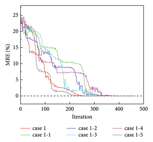
Figure 6(a) shows damage condition B, in which the damaged members were concentrated in the right region of the structure. The numbers of damaged members were 65, 69, 72, 73, 74, and 81. The “as-is” cross-sectional areas of damage condition B are listed in Table 3. Figure 6 shows different separation scenarios for damage condition B. The loading conditions in case 2 were the same as those in case 1. Figures 6(b), 6(c), 6(d), 6(e), and 6(f) show the sensor locations, and the substructure DOFs decrease with changes in the displacement sensor location. The loading points for cases 2-1 to 2-5 were at Nodes 25 and 26. External loads (10 kN) were applied in the X- and negative Z-directions of Node 25, and in the X-, negative Y-, and negative Z-directions of Node 26.

Table 3. “As-is” cross-sectional areas of damage condition B.

Damaged member	Cross-sectional area $$ (mm2)
65	2850
69	2700
72	2250
73	2100
74	2550
81	2400

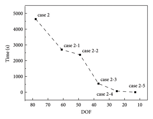
The inversion times for damage condition B were also determined. Table 4 records the inversion times under damage condition B. Figure 7 shows the inversion times for the separation cases. The related DOFs for cases 2 and 2-1 to 2-5 were 78, 61, 49, 37, 25, and 13, respectively. The results show that the inversion time decreases with the decrease of the substructure DOFs.

Table 4. Inversion times of damage condition B.

Case	Case 2	Case 2-1	Case 2-2	Case 2-3	Case 2-4	Case 2-5
Time (s)	4637.74	2701.38	2370.64	543.14	65.24	0.47

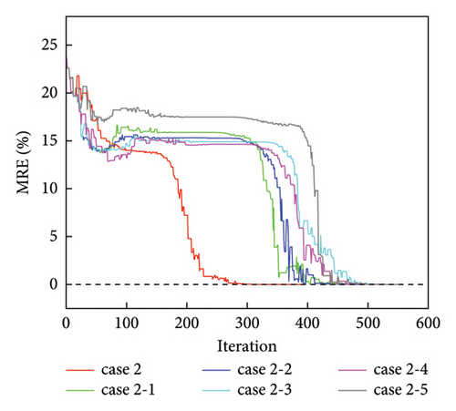
The changes in the MRE values obtained during the optimization process are shown in Figure 8. Each case’s MRE value tends to zero, and the damage has been identified accurately.

3.2. Multi-Region Damage Identification

This section presents the cases in which damage occurred in more than one region. The damage is separated into two and three regions. In these cases, each separated substructure not only had a decreased stiffness matrix dimension but also had a reduced number of unknown parameters.

For damage conditions C and D, damage occurs in two and three regions, respectively, and the loading conditions for all cases are the same as those in case 1. Figure 9(a) shows damage condition C. The damaged members are Members 2, 12, 14, 69, 73, and 74, and their “as-is” cross-sectional areas of damage condition C are listed in Table 5. The displacement sensors separated the structure into two substructures (Figures 9(b), 9(c), 9(d), and 9(e)). Each substructure contains three damaged members.

Table 5. “As-is” cross-sectional areas of damage condition C.

Damaged member	Cross-sectional area $$ (mm2)
2	2850
12	2700
14	2250
69	2400
73	1950
74	1800

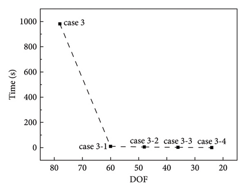
First, Table 6 shows the inversion times for cases 3 and 3-1 to 3-4. For cases 3-1 to 3-4, the inversion time was the sum of the times of the two substructures. Figure 10 illustrates the comparison of inversion time in damage condition C. The inversion times of cases 3-1 to 3-4 were significantly more reduced than case 3. For damage condition C, the damage is distributed in two regions. The DOF in a single substructure is significantly reduced when the structure is separated into two regions. Consequently, the dimensionality of the sub-stiffness matrix for inversion is significantly reduced. Besides, this example shows that separating the damage into two substructures can reduce the unknown parameters for each substructure. Even if the total number of two-regions’ unknown parameters remains unchanged, the total inversion time decreases.

Table 6. Inversion times of damage condition C.

Case	Case 3	Case 3-1	Case 3-2	Case 3-3	Case 3-4
Time (s)	981.05	9.69	5.23	2.20	0.02

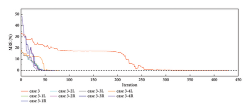
Next, all cases of damage condition C were determined. Figure 11 shows that the MRE values change with the number of iterations; L represents substructure 1, and R represents substructure 2. As shown in Figure 11, the MRE values approached zero, and the damage was identified accurately.

Obviously, case 3 required more iteration steps than the other cases (Figure 12). Figure 12 shows a comparison of the number of iteration steps between case 3 and the others. The average number of iterative steps for the separated substructure was 74, which was less than 1/5 of the iterative steps in case 1. This example indicates that reducing the unknown parameters can significantly enhance computational efficiency for identifying damage.

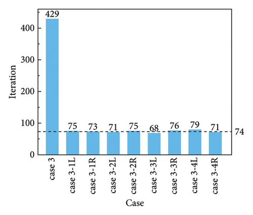
Figure 13(a) shows damage condition D, which is used to study the damage identification of the three regions. The damaged members were numbered 12, 15, 36, 39, 69, and 72. The cross-sectional areas of damage condition D are listed in Table 7. Figures 13(b) and 13(c) show the sensor locations for different separation cases. For cases 4-1 and 4-2, each substructure contains two damaged members.

Table 7. “As-is” cross-sectional areas of damage condition D.

Damaged member	Cross-sectional area $$ (mm2)
12	2700
15	2250
36	2100
39	2850
69	2550
72	2400

Figure 14 shows the inversion time for each case. The inversion time for case 4 is 1486.29 s. The inversion time for cases 4-1 and 4-2 is 1.00 s and 0.13 s, respectively. For cases 4-1 and 4-2, each inversion time was the sum of the times of the three substructures. Separating the damage into three regions can significantly improve the inversion efficiency. For damage condition D, the damage is distributed in three regions. The structure is separated into three substructures. Thus, the dimensions of the matrix for inversion in a single substructure are smaller and make the inversion more efficient.

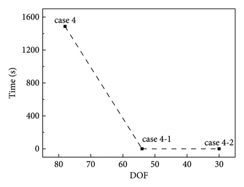
Figure 15 shows the changes in the MRE with the iterative process. The MREs of all cases eventually converged to zero. In Figure 15, L, M, and R represent Substructures 1, 2, and 3, respectively.

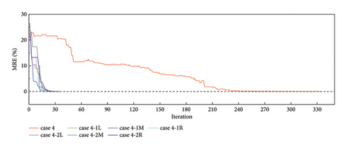
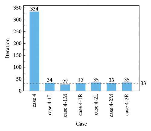
Figure 16 shows a comparison of the iteration steps for damage condition D. The average number of iteration steps for cases 4-1 (L, M, and R) and 4-2 (L, M, and R) was 33 (Figure 16), lower than 1/10 of the steps for case 4. The results from damage conditions C and D show that fewer parameters to be identified can improve optimization efficiency.

Finally, by comparing the results from signal-region damage identification, multi-region damage identification can further simplify the computational effort required for damage identification. Multi-region damage identification reduces the number of unknown parameters for each substructure, significantly enhancing the efficiency of the matrix inversion time and optimization calculations.

4. Conclusion

In summary, the stiffness separation method provides an efficient solution for quantifying damage to a large truss structure without sacrificing the accuracy of damage identification. Compared to the direct damage identification method, stiffness separation reduces the workload of inverse calculations and the computational effort in identifying truss structure damage. The inversion times of damage conditions A and B drop from 547.37 s and 4637.74 s to 0.01 s and 0.47 s, respectively. The inversion times of damage conditions C and D reduce from 981.05 s and 1486.29 s to 0.02 s and 0.13 s, respectively. In this study, the inversion times shortened as the DOFs of the substructure reduced. The multi-region damage identification results show that dividing the entire structure into several substructures can reduce the number of unknown parameters in the stiffness matrix. Even if the total number of unknown parameters remains unchanged, multi-region damage identification can significantly shorten the inversion time and improve optimization calculation efficiency. Furthermore, the method proposed in this study can be extended to other large-scale structures, such as space truss roof structures and long-span bridges. The application for different large-scale structures will be further studied. Besides, the effect of measurement errors and temperature on the proposed method will be investigated in future research.

Conflicts of Interest

The authors declare that there are no conflicts of interest.