Enhanced Multi-UAV Path Planning in Complex Environments With Voronoi-Based Obstacle Modelling and Q-Learning
Abstract
To tackle the challenge of obstacle avoidance path planning for multiple unmanned aerial vehicles (UAVs) in intricate environments, this study introduces a Voronoi graph–based model to represent the obstacle-laden environment and employs a Markov decision process (MDP) for single UAV path planning. The traditional Q-learning algorithm is enhanced by adjusting the initial state of the Q-table and fine-tuning the reward and penalty values, enabling the acquisition of efficient obstacle avoidance paths for individual UAVs in complex settings. Leveraging the improved Q-learning algorithm for single UAVs, the Q-table is iteratively refined for a fleet of UAVs, with dynamic modifications based on the waypoints chosen by each UAV. This approach ensures the generation of collision-free paths for multiple UAVs, as validated by simulation results that showcase the algorithm’s effectiveness in learning from past training data. The proposed method offers a robust framework for practical UAV trajectory generation in complex environments.
1. Introduction
With the rapid development of unmanned aerial vehicle (UAV) technology and automation, the coordinated flight of UAV swarms has emerged as a cutting-edge research area. The potential for multi-UAV coordination is immense across various fields, including panoramic photography, disaster relief, environmental monitoring, traffic surveillance, and power line inspections. In this context, path planning has become a central challenge in multi-UAV coordinated flight, concerning how UAVs can efficiently coordinate their flight, avoid collisions, and complete tasks successfully. Both academia and industry have placed significant emphasis on this issue. This paper is aimed at delving into the advancements in multi-UAV path planning research, identifying and addressing the shortcomings of existing methods, and proposing an innovative obstacle avoidance path planning strategy based on an improved Q-learning algorithm, significantly enhancing the execution efficiency and operational safety of multi-UAV coordinated flight missions.
Numerous scholars worldwide have conducted extensive research on multi-UAV path planning and achieved certain results. Literature [1] analyses various path planning techniques for UAVs over the years, emphasizing the need for path planning technologies to calculate the shortest safe path to the final destination, with the prerequisite that the path planning environment is known. Therefore, the path planning problem for UAVs inevitably accompanies the issue of environmental construction. Literature [2] summarizes various path planning strategies for autonomous underwater robots based on the predictability and unpredictability of underwater environments. Literature [3] proposes a new hybrid path planning method that combines the A∗ algorithm with an adaptive window approach for global path planning, real-time tracking, and obstacle avoidance in large-scale dynamic environments. Literature [4] creates a dynamics-constrained global-local (DGL) hybrid path planning scheme for autonomous surface vehicles (ASVs) with constrained dynamics, combining global path planning and local hierarchical architecture. By inserting virtual waypoints on the globally optimal path, it designs a seamless interface between global and local path planning mechanisms, contributing to the entire DGL hybrid path planning scheme. Literature [5] presents an autonomous path planning model based on deep reinforcement learning (DRL) to achieve intelligent path planning for unmanned ships in unknown environments. It translates navigation rules and ship encounters into navigation-restricted areas to ensure the safety of the planned path, ensuring the effectiveness and accuracy of the model. Literature [6] suggests that new path planning strategies can be developed by combining some of the strategies in the literature, a path planning platform can be developed to help select the most suitable path planning strategy with the required characteristics, future research can consider energy consumption in path planning, benchmark models can be designed for testing the performance of path planning strategies, different manufacturing characteristics can be weighed in future path planning design processes, and finally, machine learning can be a powerful tool for further improving path planning strategies. Literature [7] introduces the research progress of path planning based on multimodal constraints, which can be divided into three stages according to its basic elements (such as shape, kinematics, and dynamics): route planning, trajectory planning, and motion planning. Literature [8] studies path planning for mobile robots using neural networks and hierarchical reinforcement learning, comparing their proposed algorithm with different algorithms in path planning, and finds that the deep deterministic policy gradient (DDPG) has shorter path planning time and fewer path steps compared to double deep Q-learning (DDQN). Literature [9] addresses some of the shortcomings of the traditional ant colony optimization (ACO) in indoor mobile robot path planning, such as long path planning time, slow convergence speed, and local optimal solution characteristics, and proposes an improved adaptive ACO (IAACO). Literature [10] focuses on the path planning problem of heterogeneous UAVs in multiple areas, proposing an algorithm based on the ant colony system. Literature [11] transforms the multi-UAV cooperative control problem into a multiconstraint decision problem and describes it as a Markov decision process (MDP), laying the foundation for proposing a reinforcement learning algorithm based on global and local attention mechanisms. Literature [12] focuses on task scheduling issues, proposing a scheduling algorithm based on the energy difference coefficient to minimize energy consumption.
This paper is aimed at deeply analysing the research progress in multi-UAV path planning, identifying and addressing the shortcomings of existing methods, and proposing an innovative obstacle avoidance path planning strategy based on an improved Q-learning algorithm. Swarm intelligence algorithms such as ACO and genetic algorithms have the advantage of fast convergence but suffer from poor linearity and difficulty in portability. In contrast, reinforcement learning algorithms have strong online capabilities, wide applicability, and the ability to learn continuously. To ensure fast problem-solving and strong real-time performance, this paper proposes an innovative obstacle avoidance path planning strategy based on an improved Q-learning algorithm. The Q-learning algorithm is one of the classic algorithms in reinforcement learning, belonging to model-free algorithms, which do not require a specific environmental model. It only needs to train a policy to determine the most appropriate action to take in a given state, which is particularly suitable for obstacle path planning for multi-UAVs in complex environments due to the limited actions of UAVs and the complexity of their environment, which is difficult to model. By establishing an obstacle environment model based on Voronoi diagrams and a Markov decision model for single-UAV obstacle path planning, we improve the traditional Q-learning algorithm to enhance the performance of obstacle path planning for single UAVs in complex environments. Building upon this, we apply the improved Q-table to multiple UAVs, iteratively updating and adjusting it in real-time to achieve obstacle path planning for multi-UAVs in complex environments.
The organization of this paper is as follows: Section 1 introduces the development background of UAV technology and the importance of path planning; Section 2 elaborates on the obstacle avoidance path planning problem for multiple UAVs in complex environments; Section 3 proposes a multi-UAV path planning method based on improved Q-learning, including strategies for both single UAV and multi-UAV path planning; Section 4 validates the effectiveness of the proposed method through extensive experimental results and compares it with traditional Q-learning and Particle Swarm Optimization (PSO) algorithms; Finally, Section 5 concludes by summarizing the main contributions and research findings of this paper.
2. Problem Description of Obstacle Avoidance Path Planning for Multiple UAVs
2.1. Path Planning Background
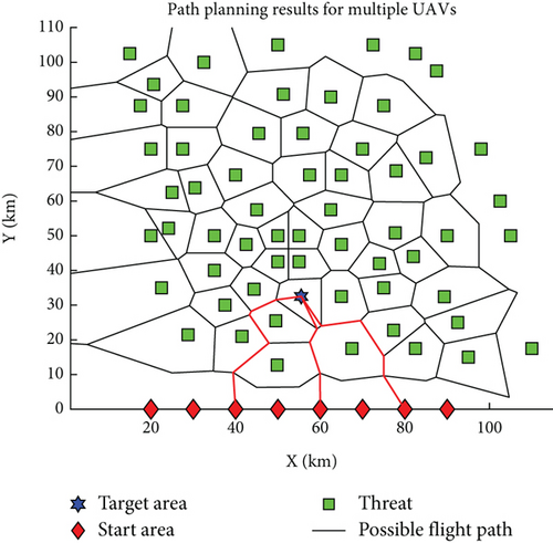
In the preparatory phase of the mission, following meticulous reconnaissance, we have identified NT critical target areas, which are surrounded by NP potential threat points, constituting the obstacles that must be cautiously avoided during the execution of the task. According to a meticulously designed operational plan, we have deployed multiple UAVs, each carrying payloads of varying specifications, taking off from their respective bases to traverse this complex airspace with the goal of safely and efficiently reaching their designated target points. The challenge of path planning lies in the UAVs’ need to navigate a route that is both short and safe while ensuring they do not trigger any threats. As depicted in Figure 1, green squares mark the locations of threat points, red diamonds indicate the starting bases of the UAVs, and blue hexagons clearly designate the target areas. Black solid lines outline the possible flight paths of the UAVs. To facilitate analysis, we assume that all UAVs possess exceptional payload capabilities and sufficient performance to undertake this formidable task.
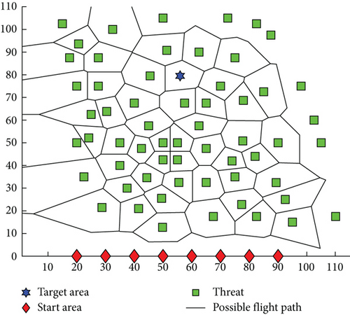
To effectively plan paths for multiple UAVs, constructing a high-quality model of the path planning space is crucial, as the model’s quality and its compatibility with the algorithm can greatly influence the success of the path planning process [13]. Among the current methods for spatial modelling, the sketch map method, grid method, and potential field method are the most prevalent [14]. The grid method breaks down the space into regular, manageable units and evaluates their connectivity to determine feasible routes. However, in environments dense with obstacles, as depicted in Figure 1, this approach can result in an overwhelming number of units, leading to extended planning times and suboptimal paths that may not accommodate the manoeuvrability required by UAVs. The potential field method offers a continuous modelling approach, known for its simplicity and computational efficiency. Yet, in complex settings, it can present local minima that may ensnare the UAV, causing the path planning to fail. Therefore, this paper adopts the sketch map method for spatial partitioning, with the Voronoi diagram emerging as the most illustrative example of this approach.
In the context of UAV path planning, the threat source set P = {P1, P2, ⋯, PNP} and the target point set T = {T1, T2, ⋯, TNT} are used as the generator points for the Voronoi diagram. The threat source set P represents the positions of threats that UAVs need to avoid, while the target point set T represents the destination of the UAVs. By constructing a Voronoi diagram, we can clearly define how UAVs can reach their destinations while avoiding obstacles.
The edge set is composed of the boundaries between obstacles and the boundaries between obstacles and target points. In the path planning space, the feasible path for UAVs is restricted to the interior regions of the Voronoi diagram, excluding any Voronoi regions. This means that UAVs only need to search for the shortest path from the starting point to the target point within these regions, ensuring that they do not cross any Voronoi boundaries, thus effectively avoiding obstacles. In this way, Voronoi diagrams provide UAVs with an intuitive and mathematically rigorous method for obstacle avoidance path planning.
2.2. Constraints
- 1.
Path feasibility: when assigning any UAV (UAVi(UAVi ∈ U = {UAV1, UAV2, ⋯, UAVNU})) to the target Tj, the planned path must be feasible, that is
- 2.
The endurance of the UAV is sufficient: the remaining navigable distance length of the UAV must be greater than the planned path length, that is
- 3.
The safety distance constraint states that the shortest distance between the trajectories of any two UAVs should be greater than the size of the UAVs, which can be mathematically expressed as
3. Multi-UAV Path Planning Method Based on Improved Q-Learning Algorithm
Multi-UAV obstacle avoidance path planning is essentially an amalgamation of two distinct challenges: obstacle avoidance path planning for a single UAV within a complex environment and collision avoidance among multiple UAVs. This approach involves a strategic progression where the initial focus is on resolving the single UAV’s obstacle avoidance in a complex setting. Subsequently, the problem shifts to addressing collision avoidance for multiple UAVs, culminating in a comprehensive solution for multi-UAV obstacle avoidance path planning. This methodical transition ensures a systematic and effective resolution of the intricate navigational challenges faced by UAV fleets.
3.1. Markov Modelling
To effectively apply the Q-learning algorithm to this problem, it is imperative to initially frame the issue within the context of Markov modelling. The MDP represents the quintessential mathematical formulation of a reinforcement learning scenario, encapsulated by a five-element tuple <S, A, {Psa}, γ, R> [15]. Within this framework, the entity responsible for learning and making decisions is termed an “agent,” while the external elements that interact with the agent constitute the “environment.” This dynamic interplay unfolds as the agent chooses actions, the environment reacts, and the agent transitions to new states [16]. Integral to this process is the environment’s provision of a “reward,” a quantifiable value that the agent aims to maximize during its decision-making, as illustrated in Figure 2.

- 1.
Represents a state set. The state set is defined by the positions that the UAV can occupy as it navigates along the path depicted in the Voronoi diagram. These positions encompass the UAV’s starting point, as well as the node and target positions within the diagram. Consequently, the state space for a single UAV consists of (1 + NV + NT) unique states, which is the sum of the number of nodes and targets in the Voronoi diagram. To prevent the UAV’s flight path from being detected, which could lead to potential harm to multiple UAVs, and given that the feasible paths in the Voronoi diagram are predetermined, the flight paths of UAVs assigned to the same target do not intersect. This ensures that the actual number of states for a single UAV is less than (1 + NV + NT), as each UAV’s path is unique and does not overlap with others.
- 2.
Represents a set of actions. The next state that the UAV can transfer to in each state is regarded as the action of the UAV; therefore, the action of the UAV in each state is different but determined, and the next state transferred to is not the same, but because the number of states of the UAV is limited, the number of actions of the UAV will not exceed the number of states, which is also different from the fixed number of actions in the traditional Q-learning algorithm. In reinforcement learning, the selection of UAV actions is a delicate balance between “exploration” and “exploitation.” Exploration involves the UAV disregarding past experiences and venturing into new behaviours at random, aiming to gather more information such as the outcomes of various actions, which contributes to the expansion of the Q-table. Conversely, exploitation is guided by accumulated experience, seeking to make the most informed decisions based on current knowledge, with the goal of refining the Q-table [17, 18]. In the training phase of this study, a strategy ε − greedy is employed to determine action selection, where actions are chosen randomly with a probability of ε to foster exploration and with a probability of 1 − ε to leverage the best-known action for exploitation, thus harnessing the benefits of prior training. A random number randt is generated with each action selection, ensuring that the action selection strategy adheres to the principles of both exploration and exploitation.
- 3.
{Psa} is the state transition probability. Psa represents the probability distribution of the current s ∈ S state that is transferred to another state after action a ∈ A. Since the action of the UAV is selected as the next state of the UAV, the probability of state transition in this paper is 1, the probability of transferring to the state corresponding to the selected action is 1, and the others are 0.
- 4.
γ ∈ [0, 1) is the discount factor. The parameter that calculates the cumulative return reflects the impact of the return at the future moment on the current moment. Larger γ indicates that greater impact and decision-makers are more focused on long-term interests, while conversely, smaller γ indicates that decision-makers are more focused on immediate interests. According to the definition of the Q-learning algorithm, the Q value update rule is satisfied.
- 5.
The payback function R(s, a, s′) represents the immediate return obtained by performing an action a in state s to move to the next state s′. In order to solve the path planning problem of a single UAV, this paper designs a return function as follows:
3.2. A Single-UAV Path Planning Method Based on Improved Q-Learning Algorithm
The steps of path planning for a single UAV based on the improved Q-learning algorithm are as follows. During initialization, “initialize all Q(s, a)” represents assigning an initial Q value to each state-action pair in the Q-learning algorithm. These values are typically initialized to zero, indicating that the expected return for any state-action combination is unknown before any experience is gained; the learning rate α is a value between 0 and 1, which controls the extent to which new information influences the update of Q values. A higher α means that new experiences have a greater impact on Q values, while a lower α implies that old experiences have a more lasting effect on Q values. A reasonable range for α is typically between 0.1 and 0.5; the maximum number of learning rounds Tmax refers to the maximum number of iterations the algorithm will execute before stopping learning. This parameter needs to be determined based on the complexity of the problem and the desired precision of learning, and in practice, it may require experimentation to find the appropriate value; the discount factor γ is a value between 0 and 1, which represents the importance of future rewards relative to current rewards. A larger γ means that future rewards are given more weight, while a smaller γ implies a greater emphasis on immediate rewards. This parameter is crucial for balancing short-term and long-term returns, and a reasonable range for γ is typically between 0.8 and 0.99; ε in ε − greedy strategy is a value between 0 and 1, used to balance exploration (exploring new state-action pairs) and exploitation (choosing the current optimal state-action pair). A smaller ε means that the algorithm is more inclined to exploit known optimal strategies, while a larger ε encourages exploration. The ε value is usually set higher at the beginning of training and gradually decreases as training progresses, ensuring that the algorithm can fully explore and ultimately converge to the optimal strategy. Algorithm 1 demonstrates the process of implementing path planning for a single UAV.
-
Algorithm 1: A single-UAV path planning method based on an improved Q-learning algorithm.
-
Input: target location information, obstacle location information, initial position information of the UAV.
-
Output: The UAV’s waypoint
-
1. According to the target position information, obstacle position information and UAV initial position information, the V map is constructed;
-
2. Initialize all Q(s, a), learning rate α, maximum number of learning rounds Tmax, discount factor γ, ε in ε − greedy strategy;
-
3. For the t-round study t = {1, 2, ⋯, Tmax}:
-
4. In the initial position state s0 of the UAV, action a is selected according to strategy ε − greedy, and the next state s1 is obtained;
-
5. If t ≤ Tmax:
-
6. Based on the current state and action, return to the next state and return;
-
7. If the next state is a terminated state:
-
8.
-
9. Otherwise:
-
10. Q(St, At)⟵Q(St, At) + (1 − α)[R − Q(St, At)]
-
11. Update the status;
-
12. According to the obtained Q table, the path point of the UAV is planned;
-
13. t = t + 1
-
14. Otherwise:
-
15. According to the obtained Q table, the path point of the UAV is planned.
- 1.
The action space is dynamically determined by the state space. Each state corresponds to a UAV position on the Voronoi diagram, with actions representing the transitions to adjacent nodes. This dependency allows the action space to be directly derived from the UAV’s state space, simplifying the Q-table by eliminating the need for a separate action space. This not only conserves memory but also streamlines the process of obtaining the UAV’s action sequence from the Q-table.
- 2.
The reward function is tailored to the UAV’s flight path. Unlike traditional reinforcement learning approaches, which often assign higher rewards to the final state and negative rewards to intermediate states to expedite learning, our algorithm considers the variable path lengths between states. This necessitates a more nuanced reward structure that not only encourages fewer state transitions but also aims to minimize the total path length of the UAV. By setting the reward as a function of the UAV’s trajectory, the algorithm incentivizes shorter, more efficient paths.
These enhancements ensure that the algorithm is better suited to the complexities of UAV path planning, particularly in environments with varying path lengths and the need for efficient navigation.
3.3. A Multi-UAV Path Planning Method Based on Improved Q-Table
If multiple UAVs depart from different bases and use the Q-learning algorithm for modelling, the status of the UAVs will increase several times, which will increase the dimension of the Q-table and increase the difficulty of searching. Considering that the environment of the UAV has not changed, the Q-table obtained by the path planning of a single UAV still has a certain feasibility when other UAVs carry out path planning, so the complex deep Q-learning algorithm is not used to solve the problem, but the changes for different UAVs are made on the basis of the Q-table obtained by the single UAV planning, so as to reduce the calculation difficulty of the UAV.
Given that the initial conditions vary among different UAVs while the planning objectives and operational environments remain consistent, each UAV must tailor the final Q-table obtained from training to its specific scenario. This involves eliminating path points previously traversed by other UAVs to prevent collisions, thereby enhancing the stealth of the UAV’s trajectory and ensuring its safety. The customized planning strategy is presented in Algorithm 2.
-
Algorithm 2: Multi-UAV path planning scheme.
-
Input: position information of NP obstacles, position information of NT targets, initial position of NU UAVs and assigned target position.
-
Output: The waypoint of the NU UAVs.
-
1. Construct the Voronoi diagram based on the positional information of obstacles and targets, as well as the initial location of the UAV, and initialize the Q-table accordingly;
-
2. For target Tk(k = 1, 2.., NT):
-
3. UAV (UAVi(i = 1, 2, ⋯)) assigned to target Tk:
-
4. Set the corresponding parameters in improved Q-learning algorithm;
-
5. The Q table was trained by the “A single UAV path planning method based on improved Q-learning algorithm.”;
-
6. For objective Tk(k = 1, 2.., NT);
-
7. UAV (UAVi(i = 1, 2, ⋯)) assigned to target Tk:
-
8. According to the results of Q table, plan the waypoint {v0, v1, ⋯}, and find the state {s0, s1, ⋯} corresponding to all waypoints (non-target points).
-
9. Update Q form: Q(:, st) = 0, (st ∈ {s0, s1, ⋯});
-
10. Return to the waypoint of the A UAV and show it in the V diagram.
4. Simulation Verification
To substantiate the efficacy and dependability of our proposed algorithm, we conducted an extensive series of simulation experiments. These experiments were designed to benchmark the performance of our enhanced Q-learning algorithm against both the conventional Q-learning algorithm and the widely recognized PSO technique. The aim was to demonstrate the superior qualities of our algorithm in terms of path planning capabilities. The simulations were executed using MATLAB R2022a (64-bit) on a Windows 11 operating system, powered by a 12th Gen Intel Core i7-12700H CPU, ensuring a robust and high-performance computing environment for the analysis.
4.1. A Multi-UAV Path Planning Method Based on Improved Q-Table
4.1.1. Parameter Setting Scheme
As per the second step outlined in Section 2.2 for the single-UAV path planning method utilizing the enhanced Q-learning algorithm, the parameters in question are α (learning rate), γ (discount factor), Tmax (maximum number of learning iterations), and ε (exploration rate).
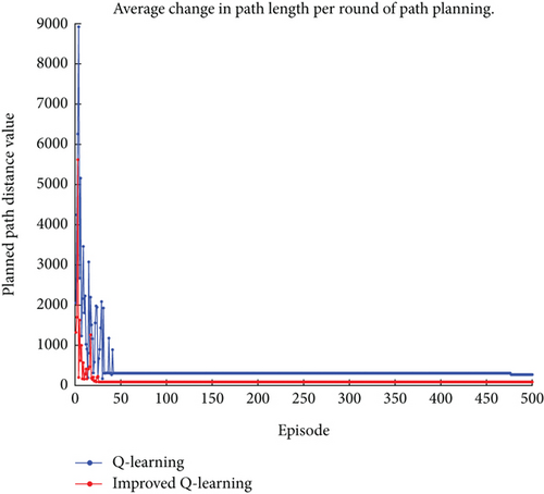
Tmax: The maximum number of learning rounds can be set to ensure that the optimal path can be planned. Let us set Tmax = 500 according to the average path length change of a single UAV per round in Figure 3. It can be seen that by improving the Q-learning algorithm, the UAV can plan the optimal path within no more than 50 learning rounds. Therefore, setting Tmax = 500 can ensure that the UAV can plan the optimal path.
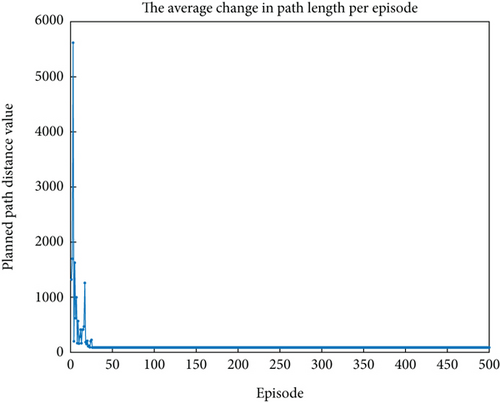
In the graph, it can be observed that the path planning length does not consistently decrease during the early stages of learning. There are occasional spikes and turning points, which occur because, in the initial phase of learning, the UAV selects actions with a certain probability at random to achieve the purpose of “exploration.” As a result, the path planning length may exhibit peaks and turning points in the early stages of learning.
α: The learning step size α ∈ (0, 1]. The smaller the step size, the more experience will be learned. However, if the step size is set too low, it will cause the UAV to rely too much on past experience during training and be unable to accumulate new rewards. Figure 4 shows the impact of A on the distance of the planned path of the UAV when α takes values between 0.1 and 0.5. It can be seen from the figure that when α = 0.36, the planned path distance is the shortest and changes relatively smoothly, so α = 0.36 is selected for the simulation.
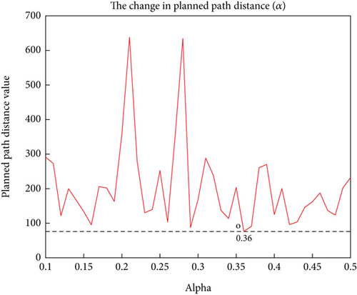
Observations from the graph indicate that as the learning rate α is adjusted, the path planning distance exhibits multiple peaks and inflection points. This phenomenon arises because when α is set to a high value, the algorithm is more inclined to accept the latest reward information, which can lead to excessive exploration in path planning. Consequently, this may result in the selection of longer or less efficient paths in certain situations, creating peaks. Conversely, when α is set to a low value, the algorithm relies more heavily on past experiences. This could cause the algorithm to react sluggishly to changes in the environment, leading to inflection points in the path planning distance during certain iterations.
γ: The discount factor γ ∈ (0, 1] reflects the influence of future rewards on the present. The larger the value, the more likely it is to learn the actions of the target state. Figure 5 shows the impact of γ taking values between 0.5 and 1 on the distance of the planned path for the UAV. As can be seen from the figure, when γ = 0.51, the planned path distance is the shortest and changes relatively smoothly. Therefore, γ = 0.51 is selected for the simulation.
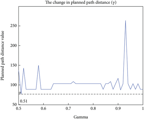
The graph reveals that as the discount factor γ is adjusted, the path planning distance exhibits several peaks and inflection points. These fluctuations are likely due to the emphasis γ places on long-term rewards within the reinforcement learning algorithm. When γ is set high, the algorithm prioritizes future rewards, which may lead to sacrificing short-term efficiency in anticipation of greater long-term gains, resulting in peaks in path planning distance. These peaks reflect the indirect or circuitous routes the algorithm might take in pursuit of the long-term optimal solution. Conversely, when γ is low, the algorithm focuses more on immediate rewards, potentially causing inflection points in the path planning distance during certain iterations, as it may become overly fixated on local optima at the expense of potentially more rewarding long-term paths.
ε: The parameter ε ∈ (0, 1] of strategy ε − greedy is used to balance the relationship between “exploration” and “utilization” during UAV training. Figure 6 shows the change in the length of the planned path of the UAV when ε takes values between 0 and 1. As can be seen from the figure, when ε = 0.36, the planned path of the UAV is the shortest, so ε = 0.36 is set.
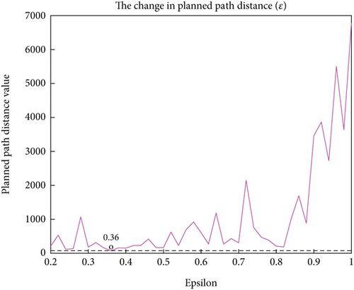
The graph illustrates that the planned path distance exhibits noticeable inflection points and peaks as the exploration rate ε varies. These fluctuations underscore the pivotal role of ε in balancing the trade-off between exploration and exploitation. When ε is set low, the algorithm favours leveraging known optimal strategies, which may result in a stable path distance over the short term, as the UAV predominantly retraces efficient paths it has already learned. However, this approach might miss opportunities to discover superior paths, leading to inflection points that signify a sudden increase in path distance. Conversely, when ε is higher, the algorithm increases the likelihood of exploring new paths, which can cause fluctuations in the path distance as the UAV temporarily deviates from the optimal solution while attempting untested routes. The peaks within these fluctuations may represent longer paths that the algorithm inadvertently discovers during exploration or reflect the uncertainty associated with trying new strategies.
4.1.2. Simulation Results
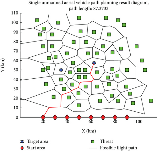
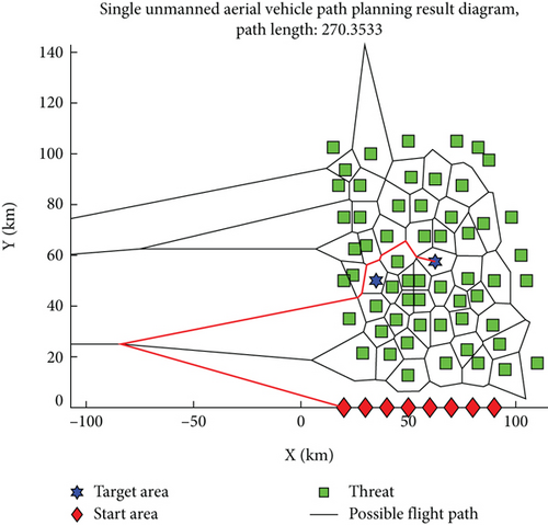
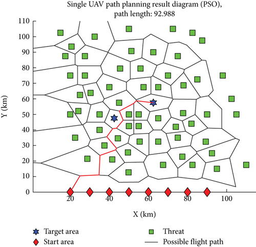
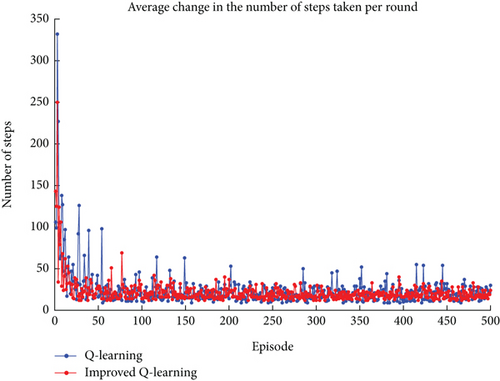
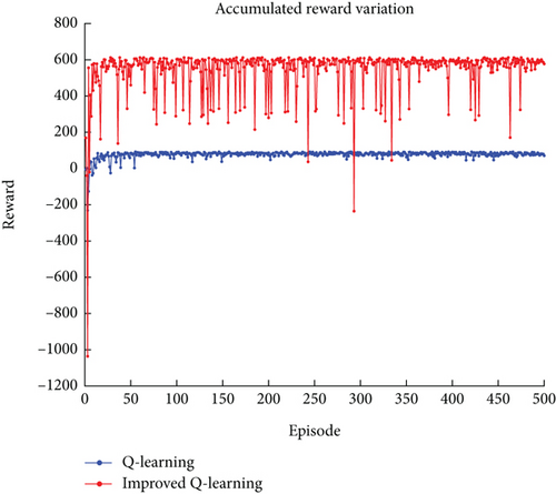
The parameter settings for the improved Q-learning algorithm and the traditional Q-learning algorithm are as follows: Tmax = 500, α = 0.36, γ = 0.51, and ε = 0.36. In the context of path planning shown in Figures 1 and 7 shows the planning result obtained using the improved Q-learning algorithm, with a planned path length of 87.3733, while Figure 8 shows the planning result obtained using the traditional Q-learning algorithm, with a planned path length of 270.3533. It can be seen that the advantage of the improved algorithm is evident, with the length of the planned path greatly reduced. However, it is worth noting that the path shown in Figure 7 has a total of 11 turns, while the path shown in Figure 8 has only 7 turns, which also confirms that linking the reward function with the UAV path can shift the focus of planning from reducing the number of learning steps to reducing the UAV path. Figure 9 shows the path planning result obtained using the PSO algorithm, with a planned path length of 92.988 and 12 turns. It can be seen that the improved Q-learning algorithm achieves better planning results compared to the PSO algorithm. Since the Q-learning algorithm is a type of reinforcement learning algorithm and the PSO algorithm belongs to swarm intelligence algorithms, it is challenging to compare the two beyond the results of their planning. Therefore, the analysis focuses on comparing the improved Q-learning algorithm with the traditional Q-learning algorithm, examining the results in terms of average path planning length per episode, average steps per episode, and cumulative reward changes as depicted in Figures 10, 11, and 12. In Figure 10, the improved Q-learning algorithm demonstrates a clear advantage over the traditional Q-learning in terms of path planning length. As the number of episodes increases, the average path planning length for improved Q-learning consistently decreases, while the reduction in Q-learning is relatively gradual. This advantage stems from the fact that the action space design in improved Q-learning is not static but varies with the current state, reducing the complexity of the space and enabling the algorithm to learn superior decision-making strategies more quickly, thus planning shorter paths in each episode. In Figure 11, the improved Q-learning algorithm shows significant superiority in reducing the average number of steps per episode. As the episodes progress, the number of steps for improved Q-learning gradually decreases, while the reduction in Q-learning is slower, indicating that improved Q-learning is more efficient in path planning and decision-making, finding the minimum number of steps required to complete tasks more rapidly. In Figure 12, the improved Q-learning algorithm exhibits a notable advantage in cumulative reward. As episodes accumulate, the cumulative reward for improved Q-learning continues to rise, while the growth of Q-learning’s reward is relatively slow, with negative growth in some stages. This advantage suggests that improved Q-learning can more effectively accumulate rewards over the long term, as the reward value in the improved algorithm varies with the planned path. Once a superior path is “explored,” the reward value is substantial, and subsequent learning processes that “exploit” this experience will also increase the reward value. Since the reward value in the traditional algorithm is fixed, the difference in reward values between the two algorithms is quite pronounced in Figure 12.
4.2. Simulation of Path Planning for Multiple UAVs
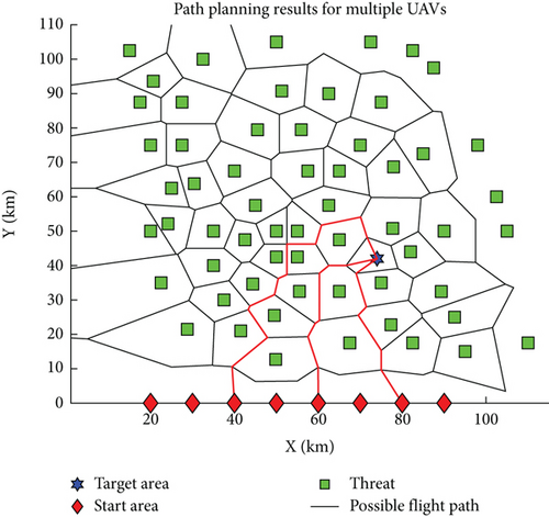
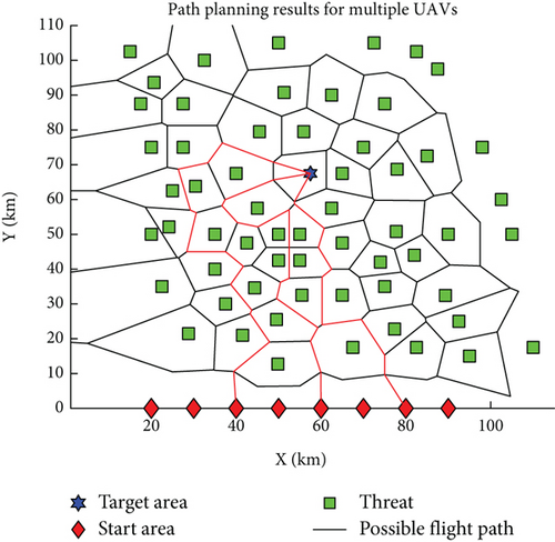
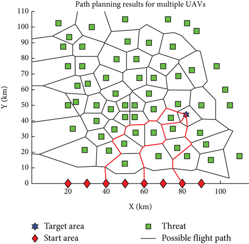
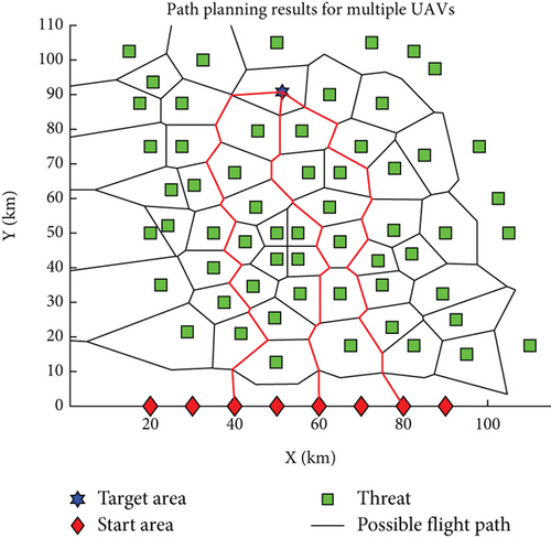
Single-UAV path planning serves as the cornerstone for multi-UAV path planning, primarily addressing issues of path feasibility and the determination of the shortest route. Building upon this, multi-UAV path planning extends to tackle the challenge of collision avoidance among multiple UAVs. Figure 13 illustrates the outcome of a multi-UAV obstacle avoidance path planning exercise, where the target is situated within a hexagonal area, and the UAVs’ starting points are all on the same side of the target. To prevent excessively long paths that may not reflect practical scenarios, path planning is conducted for three UAVs. The results depicted in Figure 13 demonstrate that the UAVs’ paths are nonintersecting, ensuring that no collisions will occur. This confirms the feasibility of employing an enhanced Q-learning algorithm for obstacle avoidance in multi-UAV systems. Figure 14 presents a scenario where the target position has been altered, showing the UAVs’ paths remain nonintersecting. This further validates the rationality and efficacy of the obstacle avoidance path planning approach, which effectively achieves the goal of safe navigation for multiple UAVs.
5. Conclusion
- 1.
The article employs Voronoi diagrams to represent the intricate environment populated with multiple UAVs, targets, and obstacles, transforming the multi-UAV obstacle avoidance path planning into a mathematically tractable problem. The objectives of multi-UAV obstacle avoidance are clearly defined within the Voronoi framework.
- 2.
By examining the relationship between the single-UAV and multi-UAV obstacle avoidance problems, the multi-UAV challenge is decomposed into two parts: the single-UAV obstacle avoidance and the multi-UAV collision avoidance. The single-UAV obstacle avoidance is further modelled as a Markov process, with the necessary Markov process elements tailored to this context, paving the way for the application of reinforcement learning algorithms to address the issue.
- 3.
A refined Q-learning algorithm is introduced for single-UAV obstacle avoidance path planning. The UAV’s action space is designed as a state-dependent variable, and a reward function is crafted to align with the planning objectives. The algorithm capitalizes on the continuous learning capabilities of reinforcement learning, thereby bolstering the reliability and practical applicability of single-UAV obstacle avoidance in complex environments. The enhanced Q-learning algorithm’s reliability and superiority are demonstrated through comparisons with the PSO algorithm and the traditional Q-learning algorithm.
- 4.
By integrating the improved Q-learning algorithm into the multi-UAV collision avoidance problem, the method iteratively refines the single-UAV obstacle avoidance path planning outcomes. The Q-table is updated dynamically based on the planned trajectories of each UAV, effectively addressing the collision avoidance challenge in complex environments. This culminates in the successful implementation of obstacle avoidance path planning for multiple UAVs, navigating through intricate scenarios with precision and efficiency.
Conflicts of Interest
The authors declare no conflicts of interest.
Funding
The authors received no specific funding for this work.
Acknowledgments
The authors have nothing to report.
Open Research
Data Availability Statement
The data used to support the findings of this study are available from the corresponding author upon request.


