International Journal of Aerospace Engineering

Volume 2024, Issue 1 4477138

Research Article

Open Access

Measurement-Driven Iterated Correction GM-PHD Filter for Passive Tracking With Hardware-in-the-Loop Simulation

Runle Du,

Runle Du

National Key Laboratory of Science and Technology on Test Physics & Numerical Mathematics , Beijing , 100076 , China

Search for more papers by this author

Jizhe Wang,

Jizhe Wang

orcid.org/0009-0009-9744-3927

School of Astronautics , Harbin Institute of Technology , Harbin , 150001 , China , hit.edu.cn

Search for more papers by this author

Di Zhou,

Corresponding Author

Di Zhou

[email protected]

orcid.org/0000-0003-0934-8882

School of Astronautics , Harbin Institute of Technology , Harbin , 150001 , China , hit.edu.cn

Search for more papers by this author

Xinguang Zou,

Xinguang Zou

School of Astronautics , Harbin Institute of Technology , Harbin , 150001 , China , hit.edu.cn

Search for more papers by this author

Jiaqi Liu,

Jiaqi Liu

National Key Laboratory of Science and Technology on Test Physics & Numerical Mathematics , Beijing , 100076 , China

Search for more papers by this author

Runle Du,

Runle Du

National Key Laboratory of Science and Technology on Test Physics & Numerical Mathematics , Beijing , 100076 , China

Search for more papers by this author

Jizhe Wang,

Jizhe Wang

orcid.org/0009-0009-9744-3927

School of Astronautics , Harbin Institute of Technology , Harbin , 150001 , China , hit.edu.cn

Search for more papers by this author

Di Zhou,

Corresponding Author

Di Zhou

[email protected]

orcid.org/0000-0003-0934-8882

School of Astronautics , Harbin Institute of Technology , Harbin , 150001 , China , hit.edu.cn

Search for more papers by this author

Xinguang Zou,

Xinguang Zou

School of Astronautics , Harbin Institute of Technology , Harbin , 150001 , China , hit.edu.cn

Search for more papers by this author

Jiaqi Liu,

Jiaqi Liu

National Key Laboratory of Science and Technology on Test Physics & Numerical Mathematics , Beijing , 100076 , China

Search for more papers by this author

First published: 24 October 2024

https://doi.org/10.1155/2024/4477138

Citations: 1

Academic Editor: Tuo Han

Share a link

Email
Wechat
Bluesky

Abstract

Considering the characteristics of Multi Aircraft Attack and Defense (MAVAD), the problem of multisensor multitarget passive tracking is researched in this article. Firstly, to solve the problem posed by incomplete or unknown knowledge about the intensity of the target’s newborns, a practical measurement–driven method of adaptive generating newborn intensity function is adopted. Then, a method named measurement–driven iterated correction Gaussian–mixture probability hypothesis density (MD-IC-GM-PHD) filter is proposed to overcome the difficulties of the observability of targets in passive tracking. Based on the above methods, a rational and efficient approach to trajectory management is presented to complete the task of recording the historical information about target states. Finally, a hardware-in-the-loop (HIL) simulation system is implemented to verify the validity of the designed multiple target tracking (MTT) algorithms.

1. Introduction

According to the detection information acquired by the sensors, MTT [1, 2] refers to the joint estimation of the number of targets in the detection area, the trajectories of the individual targets, and other characterization attributes of interest. In the scenario of MAVAD, MTT technology plays a vital role in providing information for aircraft guidance and control systems.

Due to the excellent invisibility of passive sensors, such as infrared and external radiation source radar (ERSR), passive tracking [3] become a very advantageous technique for antielectronic countermeasures, antiacoustic countermeasures, antireconnaissance, and the implementation of surprise attacks on targets. Since passive sensors can only obtain angle information from targets, it can be called bearing-only tracking. Aiming at the nonlinear problem of bearing-only tracking, extended Kalman filter (EKF), unscented Kalman filters (UKF), Gaussian sum filter, and particle filter (PF) have been utilized in many practical applications. Unfortunately, these methods cannot directly achieve MTT in MAVAD [4–6].

After years of development, the research on MTT technology has made huge progress. Based on the random finite set (RFS) theory, a series of tracking filters were proposed and researched, such as the probability hypothesis density (PHD) filter [7–9], cardinality probability hypothesis density (CPHD) filter [10], cardinality–balanced multitarget multi-Bernoulli filter (CBMeMBer) filter [11, 12]. Besides, RFS filters containing label information, like the generalized labeled multi-Bernoulli (GLMB) filter [13] and labeled multi-Bernoulli (LMB) filter [14], were derived to obtain trajectory information about targets.

To get rid of reliance on the priori intensity of the newborn, the measurement–driven target birth method is first proposed and applied on PHD/CPHD filters [15]. Then, a measurement set partition mechanism was proposed to optimize the target birth process in a high-density clutter scenario [16]. To accurately describe the state distribution of newborn targets, Reference [17] used a discrete kernel estimator and exponential weighted moving average scheme. In the field of extended target tracking, Reference [18] approximated the intensity of the newborn and potential target to β-γ-Gaussian inverse Wishart (BGGIW) mixed form. In radar long-term continuous monitoring scenarios, Reference [19] optimized the division of the measurement set and the estimation of the newborn target state distribution.

With the increasing complexity of the battlefield environment, single-sensor multiple–target tracking systems cannot satisfy the requirements of tracking accuracy and reliability anymore. Aiming at this fact, research on multiple sensor fusion systems for multiple target tracking has attracted great interest, and a series of multisensor fusion approaches appeared. Several typical filters such as the iterated corrector PHD (IC-PHD) filter, product multisensor PHD (PM-PHD), and general multisensor PHD (general PHD) were proposed by Mahler [20–22]. Considering both algorithmic performance and computational realizability, a parallel combinatorial multisensor Bernoulli–filtering algorithm was put forward by Nannuru, which used the greedy algorithm to segment the measurements and combine them with parallel filtering [22, 23]. However, the computational complexity is linearly related to the growth of the number of sensors, which causes great difficulties to practical application. In recent years, the fusion of average consensus has attracted widespread attention, including arithmetic average (AA) fusion and geometric average (GA) fusion [24, 25]. Nevertheless, both belong to the suboptimal fusion method, and the estimation accuracy may not be satisfying when the number of sensors is limited.

The trajectory management is responsible for correlating the discrete state of the target to form a complete and continuous trajectory of the target. The problem of missed detection and false alarm in MTT poses certain difficulties in accurately generating trajectories. By integrating the track management into multiple targets Bayes filter frame, labeled RFS was proposed to realize the synchronization of filtering iteration and track management [13, 26]. However, the computational complexity of these filters was too high to be applied in real engineering.

In order to reduce costs, the HIL simulation system needs to precede experimentation in the product development process [27, 28]. The risk of discovering errors in the final stage of field testing can be reduced. And it makes up for the shortcomings of the traditional software simulation that cannot accurately reproduce the actual operating conditions of complex systems; thus, HIL has been widely used in in many fields. In the field of aviation and aerospace, HIL simulation is widely implemented. Based on the data of the United States on the Patriot and Stinger missiles, HIL simulation technology has been chosen for the development of missile weapons. Its test time can be reduced by 30%–40%, and the number of test missiles can be reduced by 43.6% [29]. Some authors verified their attitude dynamics model and attitude kinematics model of satellite attitude control system with HIL simulation [30, 31]. Moreover, a multiplatform HIL was exploited to emulate the multiagent system and the communication between the UAVs, thereby reducing the risk of swarm failure [32]. Even in automotive electrification, some research about control strategy was implemented on the HIL system [33]. Inspired by them, MTT technology in the MAVAD scenario also needs to be validated by the HIL system.

In this article, the characteristics of missiles from outer space in the MAVAD scenario have been considered, which reproduced the real scene as much as possible. Cooperating with the HIL platform, an efficient and robust MTT algorithm was implemented on DSPs. Furthermore, severe dependence on initial values makes it difficult for RFS filters to be applied in actual scenarios. Due to the complex data association and optimization process during the iterative calculation, labeled RFS filters are not adopted to realize trajectory management. For practicality, the main contribution of this article can be summarized as follows:

1.
With the adaptive measurement–driven method of generating a newborn intensity function, the problem of observability of the target is solved by using multiple sensors IC-GM-PHD filter.
2.
Label–based trajectory management is proposed to overcome the difficulties of the historical association of target trajectory.
3.
The scene reconstruction method is introduced. HIL simulation is built to verify the feasibility of the proposed algorithm.

2. Preliminary Information

2.1. RFSs

In the multitarget scenario, the number of targets and their trajectories vary with time due to targets appearing and disappearing. Thus, target’s state can be modeled as a finite set of single-target state, and the MTT problem is formulated as a dynamic multitarget state estimation problem.

An RFS X is a random variable taking values of

, let X denote the multitarget state-set, so the number and value of the elements of set X are unknown and random. Due to the disorderedness of the target state and the measurement at moment k, they can be represented as follows:

()

and ℤ denotes the state space and measurement space, while

and

represents the collection of all finite subsets of

, ℤ. Targets existing at moment k − 1 in the multitarget state set X_k−1 will survive, appear, and disappear in the next moment. This process can be modeled as

()

X_k is the multitarget state set at moment k, S_k|k−1(ζ) is the spawn target sets from moment k − 1, B_k|k−1(ζ) is the RFS of survival targets, while Γ_k is the newborn target set.

Equally, measurement sets are represented as the “union” form.

()

K_k is the clutter set at time k and Θ_k(x) represents the sets of measurement from the target x. Θ_k(x) may be equal to empty set ∅ with probability 1 − p_D,k(x_k) and gain measurement with probability p_D,k(x_k).

()

2.2. GM-PHD Filters

For a RFS

, the PHD of X can be denoted by v(x). For any closed subset

, it can be obtained.

()

In the above formula, |X| is the number of elements in RFS. The physical implication of v(x) is the density of targets per unit volume at the point x, and the cardinalized estimation of RFS X is

. Furthermore, the target state can be obtained by extracting the local maximum from v(x).

By propagating the first-order statistical moment approximation of the posterior multitarget distribution, the iterative process of PHD filter can be represented as the following form:

()

where f_{k|k − 1}(x|•) is the Markov transition density, g_k(z|x) is the likelihood function, and κ_k(z) represents the density of clutter.

However, it is hard to get the analytic solution from Equation (6) directly. The core ideology of GM-PHD is to replace PDFs with the sum of a series of weighted Gaussian components (GCs) as Equation (7), and then, the solution of Equation (6) becomes available.

()

The GM-PHD filter satisfies the following assumption:

1.
The kinematic and observation model of each target can be described by the linear Gaussian dynamical model.

()

where N(x; F_k−1ξ, Q_k−1) denotes a Gaussian density with mean F_k−1ξ and covariance Q_k−1, and F_k−1 and H_k denote the state transition and measurement matrix, respectively. The process and observation noise covariance are denoted by Q_k−1 and R_k.

2.
Each target survival probability and probability of being detected are independent of the target state as

()

3.
The intensity of newborn and spawning target RFS can be represented as Gaussian mixture form as

()

Then, the complete process of PHD is as follows:

I.
Prediction

()

II.
Update

()

III.
Pruning and merging

The GCs will increase continuously during iteration. The number of GCs required to represent the intensity function v_k(x) is J_k.

()

A simple pruning process can be used to reduce the number of GCs propagating to the next time step. GCs with weights below the truncation threshold T_p can be discarded to obtain a good approximate Gaussian mixture intensity. Additionally, GCs will be merged if their Mahalanobis distances are below the threshold U. The merged GCs can be included by collection L.

()

where j is the index of the largest weight in the GC set. After merging, the weights, means, and covariances of the GCs can be obtained in the following form:

()

IV.
State extraction

The most commonly used method is to select the means of the GCs whose weights are greater than a preset threshold, as target states. According to engineering experience, the threshold is usually set to be 0.5.

2.3. Single Target Filter for Bearing-Only Measurement

The target sensor is capable of acquiring information on the orientation of the line of sight relative to the inertial coordinate at the moment of sampling, including azimuth q_β and elevation q_ε. The bearing-only measurement model is as follows:

()

where υ_k = [Δq_ε Δq_β] is the corresponding measurement noise. In the above equation,

, and

are the observation of the position coordinates of the interceptor in the three directions of the inertial coordinates of the launch point at time k.

()

Obviously, the equation cannot be used in the Kalman filter directly due to its nonlinear. Thus, according to the principle of EKF, it can be written as the following equation after local linearization.

()

Substituting Equations (19) and (20) into updating equations in an EKF, it can be able to design a single sensor filter easily.

3. Measurement–Driven Adaptive Newborn Density

3.1. Measurement–Driven Generation of Newborn GCs

According to the analysis of traditional GM-PHD trackers, if the Gaussian mixing form of the intensity function of the newborn target is given priority, the tracking performance will heavily rely on the selection of the GC of the intensity function of the “newborn.” On the contrary, the weight amplification process slows down during the measurement updating process, and it takes longer to cross the state extraction boundaries and be confirmed to be extracted. In the extreme case, the weights are progressively reduced and thus pruned, as shown in Figure 1.

Details are in the caption following the image — **Figure 1**
Open in figure viewer PowerPoint

Schematic representation of the effect of priori given newborn intensity function on the tracking effectiveness of a newborn target.

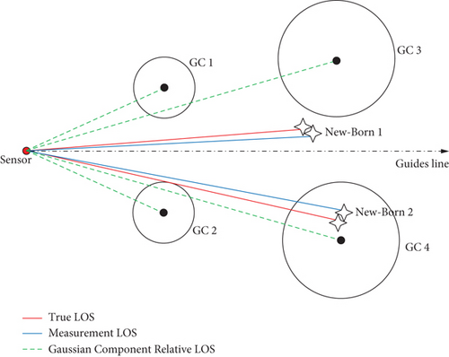
In other words, the selected newborn GCs adjacent to the truth are more likely to cross the state extraction boundaries with measurement updates. The accuracy about the target state of priority given by experience is restrictive extremely. In view of the above experience, the GM-PHD multitarget tracking driven by current measurements is proposed, which can generate the Gaussian mixture of intensity functions at the “birth point”. The specific forms are as follows:

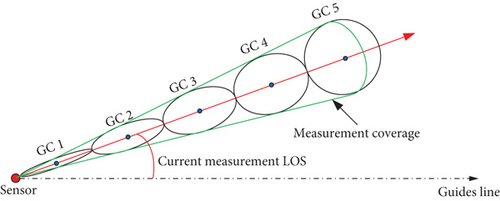
As shown in Figure 2, the form of Gaussian mixture of the intensity function of the “birth point” generated by a set of measurements from the sensors can be written as

, where

()

In the above equation, R is the detection distance with the maximum R_max and minimum R_min. N_R is the number of segments of the radial detection range. and are the measurement of LOS. δq_ε and δq_β denote the standard deviations of the measurement model. is the position of each sensor, generated by navigation module. Some constant values , , P_Vel, and are provided as a priority according to the combat performance of missiles. Through Equation (21), and can be calculated with the above parameters.

Due to the utilization of current measurement, the method is able to generate newborn intensity which has a great approximation to the probability density of a “real” newborn target. Theoretically, the performance of tracking has a positive correlation with the number of segments in the radial detection range of the detector. Thus, the denser the GCs are distributed in the radial direction, the higher the probability of gaining GCs which approach to the “real” newborn target can be obtained.

3.2. Measurement–Driven IC-GM-PHD

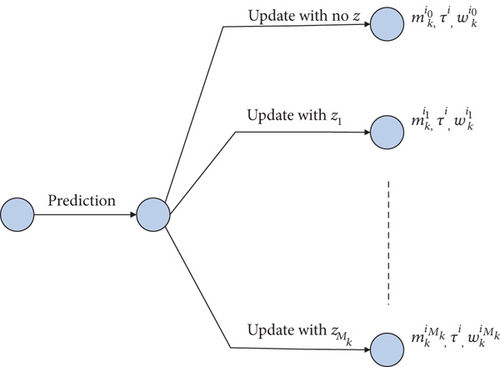
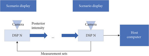
The iterative form of the PHD filter is an approximate multisensor PHD. During the update process, the measurement information received from all sensors cannot be used at the same time, so the measurement information from each sensor needs to be filtered in a certain order. As shown in Figure 3, IC-PHD includes one-step prediction and multiple PHD update processes.

To overcome the problem of observability of the target in the scenario of bearing-only detection, the principle of IC-PHD is reasonable. By updating the updated intensity function of the previous sensor, the weights of GCs belonging to the true target will increase so as to be extracted states.

The whole workflows of MD-IC-GM-PHD are as Table 1.

Table 1. Pseudocode of MD-IC-GM-PHD.

Initialization
Preset ω_γ0, R_min, R_max, N_R
New-Born Target Prediction
i = 0
for j = 1, ⋯, J_γ,k
and are generated by Equation (21)
end
Survival Target Prediction
for j = 1, ⋯, J_k−1
end
J_{k|k − 1} = i
Update
for i = 1, ⋯, N_s
for j = 1, ⋯, J_{k|k − 1}
end
l≔0
for each
l : l + 1
for j = 1, ⋯, J_{k|k − 1}
end
end
J_{k|k − 1} = lJ_{k|k − 1} + J_{k|k − 1}
end
J_k = J_{k|k − 1}

4. Label–Based Trajectory Management Method

Multitarget trajectory management algorithms can realize the historical association and vertical classification of the target state information in the time sequence. Generally, the spacing of missiles in the group is not too far. After release, missiles may overlap and separate in the sensor’s field of view (FoV). It is a huge challenge to implement the correct association of measurements and trajectories before and after rejoining and separation. To solve the problem of historical association of target trajectory, a label–based trajectory management method is presented.

On the basis of GM-PHD, GCs are labeled specifically using the following label set. τ^j is the label of the jth GCs. Each component in the prediction intensity function yields (1 + |Z_k|) GCs after measurement updating. As shown in Figure 4, the updating GCs own the same label as the prediction one.

Besides, the pruning and merging processes need to be modified as Table 2.

Table 2. Pseudocode of pruning and merging.

Preset , pruning threshold T, merging threshold U and maximum number of GCs J_max, initial l = 0,
Repeat
UntilI = ϕ
If l > J_max, then replace with J_max GCs with highest weight
Output as the pruned GCs

From the foregoing, the new labels only appear during initialization and the occurrence of the newborn GCs. Progressively, each initialized Gaussian term and each “birth point” Gaussian term acts as a root node and evolves into a tree structure with the same label (consistent with the label of the root node). As shown in Figure 5, each node of the tree structure contains information about the weights, mean, and variance of each Gaussian term at the corresponding moment. Thus, each branch of each tree structure with a specific label may represent the trajectory of a target in the FoV (historical evolutionary information of the state).

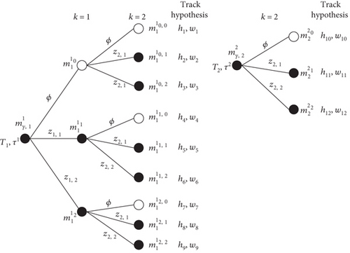
Here, n_conformed and n_missed are configured to record the number of moments when the GCs on each branch carry a weight more and less than 0.5 consecutively. indicates the boundary of the conformed initial trajectory, while indicates the boundary of the conformed terminal trajectory. The branch is recognized as a track in the FoV if , and being termination if . During the period when , the prediction of the Gaussian term of the branch node at the previous moment can be retained as a “pseudoupdated” Gaussian term at the branch node at the current moment.

5. Hardware-in-the-Loop System Simulation

In this paper, the HIL simulation system is constructed to validate the effectiveness of the algorithm in target tracking. The structure of the HIL system is shown in Figures 6, 7, 8, and 9, including three sections: target motion simulation system, target detection and tracking system, and host computer software platform.

1.
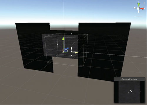
The target simulation controller displays the trajectory of the target in the FoVs on the target simulation device via Unity3d software. Each target is represented by a small circle in the FoV as shown in Figure 8. The target simulation controller solves for the FoV angle in each FoV based on the offline generated target positions. And the design sketch is shown in Figure 7.
2.
The task of the target detection system is capturing points on the screen by industrial cameras and acquiring angle information of targets through solving images. Then, each DSP executes a target-tracking algorithm regarding the measurement provided by the angle-solving module and sends the result of the algorithm to the next DSP in order to implement sequential operation. Among them, the first DSP served as the fusion center by collecting all measurement sets from other DSPs and executing new birth intensity generation.
3.
The host computer gains the trajectory information produced by the MTT algorithm, plots the trajectory dynamically, and displays the performance of the algorithm.

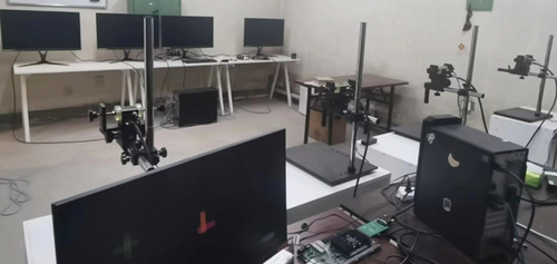
Our hardware configuration is shown in Table 3:

Table 3. Hardware list.

Image display	Dell tower workstation 7920 240 Hz high refresh rate display
Image capture and MTT	DSP TL6678F-EasyEVM TL288AP-A1 module
	MVC1381SAM-CL60-S00V0003 camera

The following experiments are performed on the HIL system. The simulation scenario is constructed as follows:

1.
Set four targets as enemy missiles and four cameras with DSPs to simulate our own side aircrafts. The initial distance between targets and aircrafts is 200 km, and the approach velocities are set to be 5 km/s. Target motion initial positions and velocities are set in Table 4:

Table 4. Initial kinematic parameters of targets.

Target	Kinematic parameters
1
2
3
4

Target motion obeys to proportional navigation (PN) guidance law which can be expressed as follows:

where

is the line-of-sight (LOS) angular rate,

is the closing velocity, and N is the navigation ratio.

To satisfy the condition of target observability, our own side aircrafts adopt the following maneuver method, whose initial positions are also set in Table 5:

2.
Parameters of the IC-GM-PHD filter are configured according to Table 6.

Table 5. Initial parameters of own side sensors.

Sensor	Kinematic parameters
1	x = −3700000 m, y = −42000 m, z = 6600000 m
2	x = −3700000 m, y = −47000 m, z = 6600000 m
3	x = −3700000 m, y = −51000 m, z = 6600000 m
4	x = −3700000 m, y = −47000 m, z = 6700000 m

Table 6. Parameters of MD-IC-GM-PHD filter.

T_f and T_m are the periods of filter and detection measuring.

, and

represent the assumed seekers’ detection area, and the clutter density is a uniform distribution over the detection area. J_max is the maximum number of GCs that could be preserved during pruning operation. T and U are the parameters used for GCs’ merging.

3.
The detection area is assumed that no clutter appears in the FoV, and only measurements generated by targets can be collected by cameras. Then, the performance of the tracking algorithm relies heavily on the qualities of detection by cameras. The angle tolerance range of camera detection is calibrated and controlled to be within average 0.5mrad. Restricted by physical conditions and the problem of sensor calibration, consistency of detection accuracy is not guaranteed.

The optimal subpattern assignment (OSPA) metric is adopted to evaluate the performance of the filters.

where the order and the cut-off value of OSPA are defined by the parameters p and c. The function variable d^(c)(x_i, y_π(i)) is the cut-off distance between the cut-off parameter c and the Euclidean distance between the states x_i and y_π(i). The set Π_n is the set of permutations with the length n, and π(i) means the ith permutation of Π_n.

Because we have labeled each trajectory, the root mean square error (RMSE) of each target can be calculated easily.

represents the estimation of jth state components, and is the real value of the state at moment k. In a Cartesian coordinate system 3D tracking scenario, target position and velocity information consist of three dimensions.

To realize communications synchronization, target detection, and tracking, the average computational times for a simulation loop period are within 15 ms.

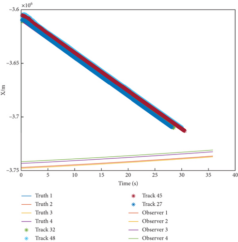
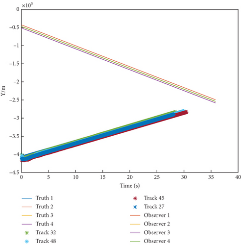
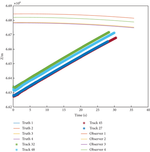
The result of trajectory tracking is displayed dynamically on the host computer during every algorithm period as shown in Figure 10. The labels of trajectory are generated randomly leading to different values in legend. For example, Track 32 corresponds to Target 1, and Track 48 corresponds to Target 2.

Figure 10 also shows the engagement scenario between the tracker and targets, the trackers execute ground attack instructions with PN guidance law, and the targets represent interceptors with a one-on-one interception strategy. The thick lines represent the truth trajectories of targets while the asterisk lines denote their estimation trajectories. Moreover, the motion paths of observers are displayed using thin lines in Figure 9. The trajectories of the targets and sensors along X-Y-Z axis are shown, respectively, in Figures 11(a), 11(b), and 11(c). As can be seen from the figure above, the asterisk lines almost cover the thick lines. This implies that the estimation tracks are very close to the truth. In order to further demonstrate the filter convergence process, Figure 12 takes the tracking path of Target 1 as an example.

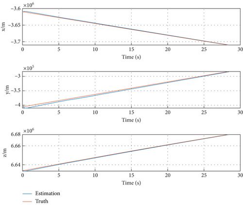
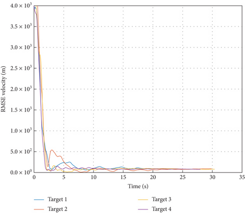
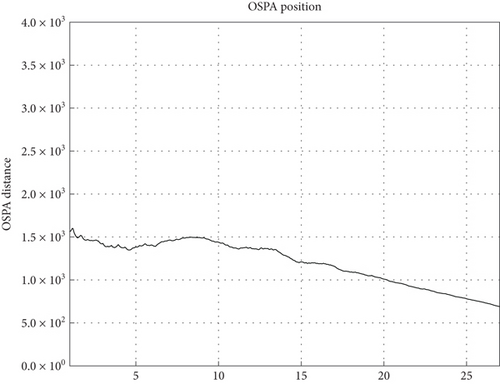
Figures 13, 14, and 15 show that MD-IC-GM-PHD is able to complete the task of target tracking in the MAVAD scenario, and tracking accuracy is within an acceptable range. The bias of state estimation mainly results from the inaccuracies of the target detection module, composed of quantization error and angular resolution error.

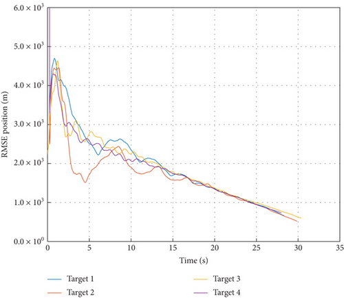
In order to conduct comparative experiments, the preconfigured newborn intensity is set in Table 7.

Table 7. Parameters of the newborn target.

It is validated that the tracking filter diverges by presetting newborn intensity under the abovementioned simulation scenario.

A different number of sensors using the mentioned measurement-driven method is adopted to perform the MTT task. OSPA distance is calculated after four groups of simulation, and the result is presented in Figure 16:

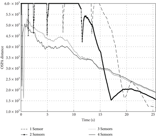
As shown in Figure 16, the convergence speed of the tracking filter positively correlated with the amount of sensors executing the MD algorithm. The reason for this is that the generation of more newborn point GCs means a higher probability of approaching the true trajectory. The simulation result is reasonable according to the analysis in Section 3.1.

6. Conclusion

In this paper, the problem of tracking multiple maneuvering targets with bearing-only measurement is considered. Considering little priori information about newborn targets in practical applications, a newborn intensity function is adaptively generated using a measurement-driven method. Compared with the traditional preparameterized approach, MD-IC-GM-PHD possesses better robustness and eliminates the need to set the initial value. Furthermore, label–based trajectory management is applied and combined with the MD-IC-GM-PHD algorithm. The convergence and effectiveness of the proposed MD-IC-GM-PHD are proved in simulation. To validate the presented algorithm, a hardware-in-the-loop simulation system was built. The design of this system highly recreates the scenario of multiaircraft countermeasures and greatly reduces the cost of experimentation. Additionally, this platform provides convenience for further research on the MTT problem.

Conflicts of Interest

The authors declare no conflicts of interest.

Author Contributions

Runle Du and Jizhe Wang contributed equally to this work.

Funding

No funds were received.

Open Research

Data Availability Statement

The data used to support the findings of this study are available from the corresponding author upon request.

References

1 Kumar M. and Mondal S., Recent developments on target tracking problems: a review, Ocean Engineering. (2021) 236, article 109558, https://doi.org/10.1016/j.oceaneng.2021.109558.
10.1016/j.oceaneng.2021.109558
Google Scholar
2 Vo B.-N., Mallick M., Bar-Shalom Y., Coraluppi S., Mahler R., and Vo B.-T., Multitarget tracking, Wiley encyclopedia of electrical and electronics engineering, 2015, Wiley, https://doi.org/10.1002/047134608X.W8275.
10.1002/047134608X.W8275
Google Scholar
3 Zhang S. Y., Xinyi H. E., and Zhang C., Present situation and prospect of underwater multi-target tracking technologies, Journal of Unmanned Undersea Systems. (2018) 26, no. 6, 511–520.
Google Scholar
4 Musicki D., Bearings only single-sensor target tracking using Gaussian mixtures, Automatica. (2009) 45, no. 9, 2088–2092, https://doi.org/10.1016/j.automatica.2009.05.008, 2-s2.0-68149148952.
10.1016/j.automatica.2009.05.008
Web of Science® Google Scholar
5 Xie Y. and Song T. L., Bearings-only multi-target tracking using an improved labeled multi-Bernoulli filter, Signal Processing.(2018) 151, 32–44, https://doi.org/10.1016/j.sigpro.2018.04.027, 2-s2.0-85046714624.
10.1016/j.sigpro.2018.04.027
Google Scholar
6 Wang Y. Y., Liu K. Z., and Feng X. S., Optimal AUV trajectories for bearings-only tracking, Robot. (2014) 36, no. 2, 179–184.
Google Scholar
7 Mahler R., Multitarget Bayes filtering via first-order multitarget moments, IEEE Transactions on Aerospace & Electronic Systems. (2003) 39, no. 4, 1152–1178P, https://doi.org/10.1109/TAES.2003.1261119, 2-s2.0-1642401353.
10.1109/TAES.2003.1261119
Web of Science® Google Scholar
8 Vo B. N., Singh S., and Doucet A., Sequential Monte Carlo methods for multitarget filtering with random finite sets, IEEE Transactions on Aerospace and Electronic Systems. (2005) 41, no. 4, 1224–1245, https://doi.org/10.1109/TAES.2005.1561884, 2-s2.0-27544460134.
10.1109/TAES.2005.1561884
Web of Science® Google Scholar
9 Vo B. N. and Ma W. K., The Gaussian mixture probability hypothesis density filter, IEEE Transactions on Signal Processing. (2006) 54, no. 11, 4091–4104, https://doi.org/10.1109/TSP.2006.881190, 2-s2.0-33747343251.
10.1109/TSP.2006.881190
Web of Science® Google Scholar
10 Mahler R., PHD filters of higher order in target number, IEEE Transactions on Aerospace and Electronic Systems. (2007) 43, no. 4, 1523–1543, https://doi.org/10.1109/TAES.2007.4441756, 2-s2.0-34347379461.
10.1109/TAES.2007.4441756
Web of Science® Google Scholar
11 Mahler R., Statistical Multisource-Multitarget Information Fusion, 2008, Artech House.
Google Scholar
12 Mahler R., Advances in Statistical Multisource-Multitarget Information Fusion, 2014, Artech House.
Google Scholar
13 Vo B. T. and Vo B. N., Labeled random finite sets and multi-object conjugate priors, IEEE Transactions on Signal Processing. (2013) 61, no. 13, 3460–3475, https://doi.org/10.1109/TSP.2013.2259822, 2-s2.0-84879315344.
10.1109/TSP.2013.2259822
Web of Science® Google Scholar
14 Reuter S., Vo B. N., and Dietmayer K., The labeled multi-Bernoulli filter, IEEE Transactions on Signal Processing. (2014) 62, no. 12, 3246–3260, https://doi.org/10.1109/TSP.2014.2323064, 2-s2.0-84901431949.
10.1109/TSP.2014.2323064
Web of Science® Google Scholar
15 Ristic B., Clark D., Vo B.-N., and Vo B.-T., Adaptive target birth intensity for PHD and CPHD filters, IEEE Transactions on Aerospace and Electronic Systems. (2012) 48, no. 2, 1656–1668, https://doi.org/10.1109/TAES.2012.6178085, 2-s2.0-84859833810.
10.1109/TAES.2012.6178085
Web of Science® Google Scholar
16 Qinling H. X., SMC-PHD/CPHD filtering for adaptive target regeneration intensity, Control and Decision. (2016) 31, no. 8, 1461–1467.
Google Scholar
17 Qiao H., Xie L., and Hongye S., Estimations of time-varying birth cardinality distribution and birth intensity in Gaussian mixture CPHD filter for multi-target tracking, Signal Processing. (2022) 190, article 108321, https://doi.org/10.1016/j.sigpro.2021.108321.
10.1016/j.sigpro.2021.108321
Google Scholar
18 Wu S., Yusong Z., Xie Y., and Qiutiao X., Robust Poisson multi-Bernoulli mixture filter using adaptive birth distributions for extended targets, Digital Signal Processing. (2022) 126, article 103459, https://doi.org/10.1016/j.dsp.2022.103459.
10.1016/j.dsp.2022.103459
Google Scholar
19 Zhao J., Zhan R., Cao J., and Peng H., Adaptive target birth intensity based on scene optimization, 2023 5th International Conference on Intelligent Control, Measurement and Signal Processing (ICMSP), 2023, Chengdu, China, 340–353, https://doi.org/10.1109/ICMSP58539.2023.10170916.
10.1109/ICMSP58539.2023.10170916
Google Scholar
20 Mahler R., The multisensor PHD filter: I. General solution via multitarget calculus, Proceedings of SPIE-Signal Processing, Sensor Fusion, and Target Recognition XVIII, 2009, Orlando, FL, USA, https://doi.org/10.1117/12.818024.
10.1117/12.818024
Google Scholar
21 Mahler R., Approximate multisensor CPHD and PHD filters, 13th International Conference on Information Fusion, 2010, Edinburgh, UK.
Google Scholar
22 Nannuru S., Blouin S., Coates M., and Rabbat M., Multisensor CPHD filter, IEEE Transactions on Aerospace and Electronic Systems. (2016) 52, no. 4, 1834–1854, https://doi.org/10.1109/TAES.2016.150265, 2-s2.0-84997606245.
10.1109/TAES.2016.150265
Web of Science® Google Scholar
23 Saucan A., Coates M. J., and Rabbat M., A multisensor multi-Bernoulli filter, IEEE Transactions on Signal Processing. (2017) 65, no. 20, 5495–5509, https://doi.org/10.1109/TSP.2017.2723348, 2-s2.0-85023173303.
10.1109/TSP.2017.2723348
Web of Science® Google Scholar
24 Üney M., Clark D. E., and Julier S. J., Distributed fusion of PHD filters via exponential mixture densities, IEEE Journal of Selected Topics in Signal Processing. (2013) 7, no. 3, 521–531, https://doi.org/10.1109/JSTSP.2013.2257162, 2-s2.0-84877917916.
10.1109/JSTSP.2013.2257162
Web of Science® Google Scholar
25 Li T. C., Corchado J. M., and Sun S. D., On generalized covariance intersection for distributed PHD filtering and a simple but better alternative, 2017 20th International Conference on Information Fusion (Fusion), 2017c, Xi′an, China, https://doi.org/10.23919/ICIF.2017.8009732, 2-s2.0-85029417335.
10.23919/ICIF.2017.8009732
Google Scholar
26 Vo B. N., Vo B. T., and Phung D., Labeled random finite sets and the Bayes multi-target tracking filter, IEEE Transactions on Signal Processing. (2014) 62, no. 24, 6554–6567, https://doi.org/10.1109/TSP.2014.2364014, 2-s2.0-84913582870.
10.1109/TSP.2014.2364014
Web of Science® Google Scholar
27 Lu B., Wu X., Figueroa H., and Monti A., A low-cost real-time hardware-in-the-loop testing approach of power electronics controls, IEEE Transactions on Industrial Electronics. (2007) 54, no. 2, 919–931, https://doi.org/10.1109/TIE.2007.892253, 2-s2.0-34247161863.
10.1109/TIE.2007.892253
Web of Science® Google Scholar
28 Issermann R., Schaffnit J., and Sinsel S., Hardware-in-the-loop simulation for the design and testing of engine-control systems, Control Engineering Practice. (1999) 7, no. 5, 643–653, https://doi.org/10.1016/S0967-0661(98)00205-6, 2-s2.0-0032628973.
10.1016/S0967-0661(98)00205-6
Google Scholar
29 Faithfull P. T., Ball R. J., and Jones R. P., An investigation into the use of hardware-in-the-loop simulation with a scaled physical prototype as an aid to design, Journal of Engineering Design. (2001) 12, no. 3, 231–243, https://doi.org/10.1080/095448201155565, 2-s2.0-0041025604.
10.1080/095448201155565
Google Scholar
30 Qiao L., Zhang M., and Osborne B., Attitude determination and control system (ADCS) of UNSW QB50 project“UNSW EC0”, Proceedings of the 13th Australian Space Science Conference, Sydney, Australia. (2013) 24, no. 1, 31–36.
Google Scholar
31 Ure N. K., Kaya Y. B., and Inalhan G., The development of a software and hardware-in-the-loop test system for ITU-PSAT II nano satellite ADCS, 2011 Aerospace Conference. (2011) 24, no. 1, 31–36.
Google Scholar
32 Khaliq S., Ahsan S., and Nisar M. D., Multi-platform hardware in the loop (HIL) simulation for decentralized swarm communication using ROS and GAZEBOn, 2021 IEEE 22nd international symposium on a world of wireless, Mobile and multimedia networks (WoWMoM), 2021, Pisa, Italy, 310–315, https://doi.org/10.1109/WoWMoM51794.2021.00057.
10.1109/WoWMoM51794.2021.00057
Google Scholar
33 Yang L., Wang W., Yang C., Du X., Liu W., Zha M., and Liang B., A self-triggered MPC strategy with adaptive prediction horizon for series hybrid electric powertrains, in IEEE Transactions on Industrial Informatics. (2024) 20, no. 4, 6762–6771, https://doi.org/10.1109/TII.2024.3353347.
10.1109/TII.2024.3353347
Google Scholar

Citing Literature

All articles

Measurement-Driven Iterated Correction GM-PHD Filter for Passive Tracking With Hardware-in-the-Loop Simulation

Abstract

1. Introduction