Analysis of the Stability and Chaotic Dynamics of an Ecological Model
Abstract
Modelling has become an eminent tool in the study of ecological systems. Ecological modelling can help implement sustainable development, mathematical models, and system analysis that explain how ecological processes can promote the sustainable management of resources. In this paper, we also chose a four-dimensional discrete-time Lotka–Volterra ecological model and analyzed its dynamic behavior. In particular, we derived the parametric conditions for the existence of biologically feasible solutions and the stability of the fixed points. We also provided graphs to study the spectrum behavior of all fixed points. In addition, we have seen that when the intrinsic dynamics of the population exceed a certain threshold, the system bifurcates. This particular range of inherent population dynamics depends on the values of other biological parameters and the initial population. We proved that the instability of the model resulted in Neimark–Sacker and period-doubling bifurcations. To confirm these two types of bifurcation, we used bifurcation theory, and to find the direction of bifurcation, we used graphical results. Mainly, through novel periodic plots, we confirm the coexistence of the population and the possible equilibrium states. We apply Marotto’s theorem to verify the existence of chaos in the system. To control the chaos, we use a hybrid control feedback methodology. Finally, we provide numerical examples to illustrate our theoretical results. The outcomes of the numerical simulations show chaotic long-term behavior across an extensive range of parameters.
1. Introduction
Population dynamics is one of the dominant themes in ecology. To discuss the dynamic relationship between the population and the ecosystem, we have two critical models. The first is a differential logistic model for a one-species ecosystem, which can explain an observed saturation phenomenon of an ecosystem’s population. The second is the Lotka–Volterra population dynamics model, which incorporates interpopulation competition in a predator-prey ecosystem. The prominent Lotka–Volterra model was introduced by Lotka [1] and Volterra [2] and has been broadly scrutinized in the literature and applied to many ecological and population dynamics. Especially in the last few decades, the Lotka–Volterra and predator-prey models have greatly interested many scientists, mathematicians, and ecologists. By modifying the Lotka–Volterra model, several critical ecological models and crucial results about these ecological models were obtained. For example, some researchers introduced new ecological models by introducing some effects in Lotka–Volterra models, which describe ecological population dynamics in a better and more detailed manner. Here are some of these effects. In the case of limited resources, the competition between a predator and prey is called the crowding effect. For a detailed study of the predator-prey model with the crowding effect, we refer the interested readers to references Abbasi and Din [3] and Dhar et al. [4]. The consumption rate of a consumer is a function of density and is called a functional response, and there are three main functional responses known as Holling’s type I, II, and III [5]. For a detailed discussion about the Holling type functional response, we refer to Rosenzweig and MacArthu [6]. The ecological interaction between more than one species for the sake of net benefit is called mutualism (for details, see Bronstein [7]). The representation of prey consumption assuming a given number of predators is known as the trophic function. A detailed study with trophic function is in references Rai et al. [8] and Buffoni et al. [9]. The fear of being preyed upon by the predator is called the fear effect. The fear effect has a profound impact on the growth of the prey population. For a detailed study of the fear effect, we recommend references Abbasi and Samreen [10]; Abbasi [11]; Tian and Li [12]; and the references therein.
Initially and most commonly, the Lotka–Volterra model is studied in differential equations representing continuous-time dynamics. Still, in a natural ecosystem, populations of each species cannot occur continuously because of competitive interaction. Moreover, nearly all ecological species have essential life-history components in discrete forms, such as synchronized breeding seasons and seasonal deaths. Also, the discrete models effectively represent complex ecological processes; they clarify population cycles, such as the relationship between the snowshoe hare and the lynx. They play a crucial role in comprehending phenomena, including the spread of invasive species, disease transmission dynamics, and conservation planning. They offer insightful information essential for efficient ecosystem management and conservation activities. Therefore, using a discrete-time dynamical system is more suitable for populations in the natural ecosystem. Considering the importance of difference models, ecologists and mathematicians use difference equations to study the ecological populations’ qualitative behavior and model their behaviors. Furthermore, due to rich dynamical behavior, discrete-time models have gained more and more attention in recent years, like complex behavior in the neighborhood of the equilibria, bifurcation, chaos, global properties, periodicity, graphical and algebraic techniques, bounded solution trajectories, and more perfect numerical simulation results in. These discrete ecological models include predator-prey models, plant-herbivore models, Lotka–Volterra models in their modified form, host-parasitoid models, and many more. Interested readers can find some essential results related to the dynamics of the discrete-time models in references Mokni and Ch-Chaoui [13]; Mokni et al. [14]; and Ran and Zhou [15]. In reference Mokni and Ch-Chaoui [13], the authors discussed the dynamics of the discrete model incorporating the immigration effect. They showed interesting results on how immigration affects the dynamics of the model. Mokni et al. [14] included the Holling type III functional response to the predator-prey model and discretized the model using a nonstandard finite difference scheme. They found that the model is dynamically rich, showing different types of bifurcation. Similarly, more recent results related to the discrete-time models can be found in Ran and Zhou [15]. Some more interesting results about these discrete-time models are as follows. The plant-herbivore model is a modified form of the predator-prey model. For the dynamical behavior, stability of equilibria, period-doubling bifurcation, Neimark–Sacker bifurcation, transcritical bifurcation, homoclinic bifurcation, chaos control, and limit cycles for different discrete-time plant-herbivore ecological models, we refer to Kang et al. [16]; Kartal [17]; Li et al. [18]; Liu et al. [19]; Din [20]; Din [21]; and Elsayed and Din [22]. The organisms that depend on the hosts and kill them sooner or later are called parasitoids. The host-parasitoid ecological models are used to discuss the behaviors of hosts and parasitoids, and they also have a close likeness with the Lotka–Volterra models. For some recent work on the host-parasitoid model, we have Din [23]; Din and Hussain [24]; Din and Saeed [25]; and Din [26]. The ecological interaction in which one organism eats another organism is called perdition. The predator-prey models are used to discuss the perdition effect of the organism in ecology. For interested readers, some recent work on predator-prey models is cited as Din [27]; Din [28]; Din [20]; Shabbir et al. [29]; Saeed et al. [30]; and Abbasi [31]. The dispersal of living organisms is the process by which species of living organisms expand space. Dispersal can be a response to temporal heterogeneity and deteriorating local conditions [32]. The travel of the ecological population can be analyzed with dispersal models. Here are some discrete-time models to study the effects of population dispersal: Wu and Cui [33]; Lutscher and Petrovskii [34]; Ramanantoanina et al. [35]; and Yakubu [36]. Similarly, the SIR models are used to study the effects of diseases in an ecological population Hu et al. [37]; Du et al. [38]; D’Innocenzo et al. [39]. Dubey et al. [40]; Din [41]; Fan et al. [42]. Further exciting insights into the dynamics of interactions between different species that deepen our knowledge of population dynamics and evolutionary processes are available in Rael et al. [43], Din [23], Chen and Shi [44], Din [45], Din et al. [46], Mokni et al. [47], and Mokni et al. [14]. These articles provide important insights into population dynamics and evolutionary processes by exploring evolutionary game theory and applying new mathematical techniques to discrete-time models, deepening our understanding of four-dimensional systems.
Our model has the following limitations. (1) Our model captures limited biological realism. We do not consider the more realistic biological factors like intraspecific competition. (2) We do not consider spatial dynamics like migration and heterogeneity. (3) We do not consider any time delay to our model; however, in a natural ecosystem, there can be delays between changes in one population and their effects on another. (4) The model presupposes a homogeneous environment where every species member lives under the same circumstances. In actuality, habitats are frequently diverse, which causes population dynamics to vary geographically. Our model can better represent the complex nature of predator-prey interactions and offer improved predictions of population dynamics in ecological systems by overcoming these flaws and adding greater biological realism.
The article provides a detailed analysis of a four-dimensional ecological model, which increases our understanding of ecological dynamics. In the stability analysis, we use complex novel graphs to comprehend the topological classification of equilibria. We also provide novel results related to the existence of biologically feasible solutions. We use Marotto’s theorem to show the existence of chaos in the system and use a hybrid control method to control the chaos. Also, we use different novel periodic plots to confirm the equilibrium states and coexistence of populations. In the future study, we will update the model and will discuss the dynamics of the updated model. The existence of the periodic behavior of the model mathematically will also be addressed in future studies.
First, we will prove the existence of biologically feasible solutions for the system described above. For mathematical biology models to be ecologically realistic and helpful, they must show that they have biologically plausible solutions. Thus, we have the following theorem.
2. Existence of Biologically Feasible Solutions
Next, let (Y1(0), Y2(0), Z1(0), Z2(0)) ∈ D; then Yi(n), Zi(n) ≥ 0 for i = 1, 2 and for each if F(D) = D.
We will now discuss the fixed point’s existence and uniqueness. For this, we have the following lemmas.
Lemma 1. The parameters α, β, γ, δ, θ and ψ are positive iff the following conditions hold:
The following lemma shows that the positive fixed point of system (1) is unique.
Lemma 2. Assume that (α, β, γ, δ, θ, ψ) > 0; also k1r22α + δγ > βk2r12 and ψγ + k2r11β > k1r21α; then there exists a unique positive fixed point of system (1).
Proof. The fixed point of system (1) can be obtained through solving the subsequent set of equations.
Solving the last two equations of the system as mentioned above, we get
By putting these values on the first two equations of system (12), one can get
Solving these equations, we get
Therefore, system (1) has a unique fixed point which is given below:
3. Local Stability of Fixed Points
We have the following lemmas regarding the stability analysis of other fixed points. See Eladyi [50] for more details.
Lemma 3. Fixed point E0(0, 0, 0, 0) of system (1) is
- (1)
Sink if |p1| < 1, |p2| < 1, |q1| < 1 and |q2| < 1,
- (2)
Saddle if at least one and at most three of the parameters (p1, p2, q1, q2) have an absolute value greater than one and the rest of the parameters have a value less than one,
- (3)
Source if |p1| > 1, |p2| > 1, |q1| > 1 and |q2| > 1,
- (4)
Hyperbolic if |p1| ≠ 1, |p2| ≠ 1, |q1| ≠ 1 and |q2| ≠ 1,
- (5)
Nonhyperbolic if any one of the parameter {p1, p2, q1, q2} has value equal to one.
Proof. The Jacobian matrix of system (1) evaluated at the fixed point E0(0, 0, 0, 0) is given as
The latent roots of (21) are λ1 = p1, λ2 = p2, λ3 = −q1, and λ4 = −q2. The spectrum of the Jacobian matrix J1 is given as
Therefore, E0 is stable when {p1, p2, q1, q2} ∈ (0, 1) and unstable when {p1, p2, q1, q2} > 1. A detailed analysis of the behavior of the spectrum σ(E0) can be analyzed from Figure 1.
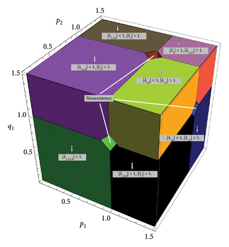
Lemma 4. Suppose that αa = (q1 − 1)k1 + s11/s11, αb = (q2 − 1)k1 + s21/s21, αc = (q1 + 1)k1 + s11/s11, αd = (q2 + 1)k1 + s21/s21, andp1 > 1. Then the equilibrium point E1(p1 − 1/k1, 0, 0, 0) of system (1) is a
- (1)
Sink if max{1, αa, αb} < p1 < min{3, αc, αd} and |p2| < 1,
- (2)
Saddle if at least one and at most three of the eigenvalues have absolute values greater than one and the rest of the parameters have values less than one,
- (3)
Source if |p1| > max{3, αc, αd} and |p2| > 1,
- (4)
Hyperbolic if |p2| ≠ 1, p1 ≠ 3, p1 ≠ αa, p1 ≠ αb, p1 ≠ αc and, p1 ≠ αd,
- (5)
Nonhyperbolic if either |p2| = 1 or p1 = 3 or p1 = αa or p1 = αb or p1 = αc or p1 = αd.
Proof. The Jacobian matrix of system (1) computed at the fixed point E1(p1 − 1/k1, 0, 0, 0) is given as
The latent roots of (23) are given as λ1 = 2 − p1, λ2 = p2, λ3 = (p1 − 1)s11/k1 − q1, and λ4 = (p1 − 1)s21/k1 − q2. Hence, the spectrum of E1 is
The fixed point E1 of system (1) is locally asymptotically stable if the spectral radius is less than one, which is possible only when max{1, αa, αb} < p1 < min{3, αc, αd} and |p2| < 1. The fixed point E1 of system (1) is unstable if spectral radii are greater than one or if every root of the characteristic function of (23) has an absolute value greater than one, which is possible only when |p1| > max{3, αc, αd} and |p2| > 1. The spectrum classification of E1 is given in Figure 2.
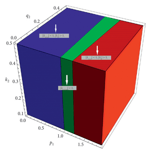
Lemma 5. Suppose that αe = (q1 − 1)k2 + s12/s12, αf = (q2 − 1)k2 + s22/s22, αg = (q1 + 1)k2 + s12/s12, αh = (q2 + 1)k2 + s22/s22, and p2 > 1. Then the fixed point E2(0, p2 − 1/k2, 0, 0) of system (1) is a
- (1)
Sink if max{1, αe, αf} < p2 < min{3, αg, αh} and |p1| < 1,
- (2)
Saddle if at least one and at most three of the eigenvalues have absolute values greater than one and the rest of the parameters have values less than one,
- (3)
Source if |p2| > max{3, αg, αh} and |p1| > 1,
- (4)
Hyperbolic if |p1| ≠ 1, p2 ≠ 3, p2 ≠ αe, p2 ≠ αf, p2 ≠ αgand, p2 ≠ αh,
- (5)
Nonhyperbolic if either |p1| = 1 or p2 = 3 or p2 = αe or p2 = αf or p2 = αg or p2 = αh.
Proof. The Jacobian matrix of system (1) calculated at the fixed point E2(0, p2 − 1/k2, 0, 0) is given as
The latent roots of the J2 are given as λ1 = p1, λ2 = 2 − p2, λ3 = (p2 − 1)s12/k2 − q1, and λ4 = (p2 − 1)s22/k2 − q2.
The spectrum of the Jacobian matrix J1 is given as
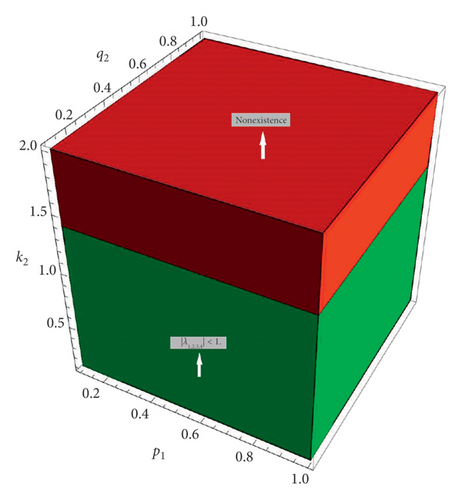
Using the above-listed latent roots, one can easily calculate that the fixed point E2 is locally asymptotically stable if the conditions listed below satisfy:
The boundary fixed point E2 is unstable if
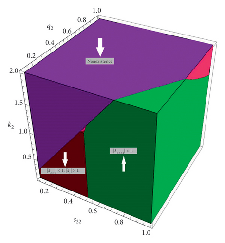
Figure 3 is the plot for the spectrum analysis of fixed point E2 in which the source and the saddle for selected parametric values can be seen.
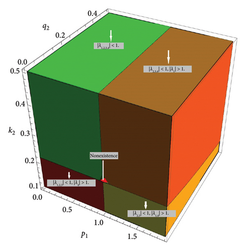
Lemma 6. Let p1 > 1, p2 > 1, αi = k1k2q1 + k2s11 + k1s12, αj = k2s11p1 + k1s12p2, αk = k1k2q2 + k2s21 + k1s22, and αl = k2s21p1 + k1s22p2; then E3(p1 − 1/k1, p2 − 1/k2, 0, 0) of (1) is a
- (1)
Sink if 1 < p1 < 3, 1 < p2 < 3, αi − k1k2 < αj < αi + k1k2 and αk − k1k2 < αl < αk + k1k2,
- (2)
Source if p1 > 3, p2 > 3, αj > αi + k1k2 and αl > αk + k1k2.
Proof. The Jacobian matrix J3 of system (1) calculated at the boundary fixed point E3(p1 − 1/k1, p2 − 1/k2, 0, 0) is given as
The spectrum of E3 is
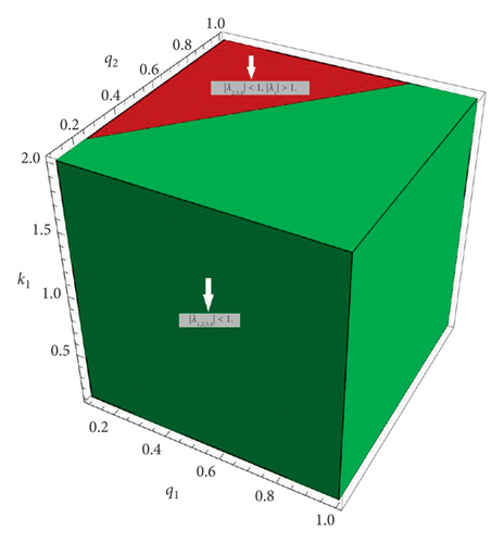
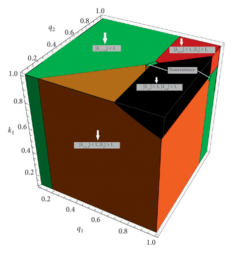
The topological analysis of set σ(E3) in graphical form is given in Figure 4.
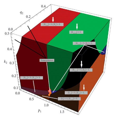
Lemma 7. Let p2 > 1 and (p2 − 1)s12 > k2(q1 + 1); then the boundary fixed point E4(0, q1 + 1/s12, (p2 − 1)s12 − k2(q1 + 1)/r21s12, 0) of system (1) is a
- (1)
Sink if |λ1,2,3,4| < 1,
- (2)
Saddle if at least one and at most three of the eigenvalues have absolute values greater than one and the rest of the parameters have values less than one,
- (3)
Source if |λ1,2,3,4| > 1,
- (4)
Hyperbolic if with |λ1| ≠ 1, |λ2| ≠ 1, |λ3| ≠ 1, and |λ4| ≠ 1,
- (5)
Nonhyperbolic if and either |λ1| = 1, |λ2| = 1, |λ3| = 1, or |λ4| = 1.
Proof. At the fixed point E4(0, q1 + 1/s12, (p2 − 1)s12 − k2(q1 + 1)/r21s12, 0), the Jacobian matrix J4 of system (1) is
Lemma 8. Let p1 > 1 and (p1 − 1)s21 > k1(q2 + 1); then the boundary fixed point E5(q2 + 1/s21, 0, 0(p1 − 1)s21 − k1(q2 + 1)/r12s21) of system (1) is a
- (1)
Sink if |λ1,2,3,4| < 1,
- (2)
Saddle if at least one and at most three of the eigenvalues have an absolute value greater than one and the rest of the parameters have a value less than one,
- (3)
Source if |λ1,2,3,4| > 1,
- (4)
Hyperbolic if along with |λ1| ≠ 1, |λ2| ≠ 1, |λ3| ≠ 1, and |λ4| ≠ 1,
- (5)
Nonhyperbolic if and either |λ1| = 1, |λ2| = 1, |λ3| = 1, or |λ4| = 1.
Proof. The Jacobian matrix J5 of system (1) evaluated at the boundary fixed point E5(q2 + 1/s21, 0, 0(p1 − 1)s21 − k1(q2 + 1)/r12s21) is given by
Lemma 9. Let p2 > 1 and (p2 − 1)s22 > k2(q2 + 1); then the boundary fixed point E6(0, q2 + 1/s22, 0, (p2 − 1)s22 − k2(q2 + 1)/r22s22) of system (1) is a
- (1)
Sink if |λ1,2,3,4| < 1,
- (2)
Saddle if at least one and at most three of the eigenvalues have absolute values greater than one and the rest of the parameters have values less than one,
- (3)
Source if |λ1,2,3,4| > 1,
- (4)
Hyperbolic if along with |λ1| ≠ 1, |λ2| ≠ 1, |λ3| ≠ 1, and |λ4| ≠ 1,
- (5)
Nonhyperbolic if and either |λ1| = 1, |λ2| = 1, |λ3| = 1, or |λ4| = 1.
Proof. The Jacobian matrix J6 of system (1) evaluated at the boundary fixed point E6(0, q2 + 1/s22, 0, (p2 − 1)s22 − k2(q2 + 1)/r22s22) is given by
Lemma 10. Let p1 > 1 and (p1 − 1)s11 > k1(q2 + 1); then the boundary fixed point E7(q1 + 1/s11, 0, (p1 − 1)s11 − k1(q1 + 1)/r11s11, 0) of system (1) is a
- (1)
Sink if |λ1,2,3,4| < 1,
- (2)
Saddle if at least one and at most three of the eigenvalues have absolute values greater than one and the rest of the parameters have values less than one,
- (3)
Source if |λ1,2,3,4| > 1,
- (4)
Hyperbolic if along with |λ1| ≠ 1, |λ2| ≠ 1, |λ3| ≠ 1, and |λ4| ≠ 1,
- (5)
Nonhyperbolic if and either |λ1| = 1, |λ2| = 1, |λ3| = 1, or |λ4| = 1.
Proof. The Jacobian matrix J7 of system (1) evaluated at the boundary fixed point E7(q1 + 1/s11, 0, (p1 − 1)s11 − k1(q1 + 1)/r11s11, 0) is given by
4. Bifurcation Analysis
Analyzing bifurcations in ecological models provides essential insights into the critical points where system behavior changes. Finding these bifurcation points helps us understand how ecosystems change from stable to chaotic states, which helps us develop ecological management and preservation strategies. We can predict and adapt to sudden changes in environmental dynamics through bifurcation analysis. Tracing bifurcation in ecological models aids in predicting and comprehending abrupt changes in ecosystems, assisting adaptive preservation and control operations. In this section, we will discuss the criteria for the existence of Neimark–Sacker and period-doubling bifurcation of system (1) at the fixed point . The period-doubling bifurcation is a process in nonlinear dynamics when the behavior of a system changes from periodic oscillations to rapidly complicated and doubled periods as a control parameter is gradually changed, while the dynamics of a system change from a stable equilibrium to continuous oscillations as a parameter crosses a crucial threshold, signifying a significant qualitative change in its behavior in a Neimark–Sacker bifurcation. This bifurcation results in closed, invariant circles. First, we present the theory for the study of Neimark–Sacker bifurcation. The criteria for studying Neimark–Sacker bifurcation with and without eigenvalues are as follows.
4.1. Neimark–Sacker Bifurcation by Finding the Eigenvalues
Lemma 11. Consider an n-dimensional map xk+1 = fμ(xk) where xk+1, xk ∈ Rn, represents the state vector, k is the iterative index, and μ ∈ R is a parameter. Assume that fμ has a fixed point x0 and satisfies the following.
- C1
Eigenvalue assignment: the Jacobian matrix has a pair of complex conjugate eigenvalues λ1(μ) and with |λ1(μ)| = 1 at μ = μ0 and the others λj(μ), j = 3, …, n, with λj(μ0) < 1.
- C2
Transversality condition: d|λ1(μ0)|/dμ ≠ 0.
- C3
Nonresonance condition: , or resonance condition: .
Then, a Hopf bifurcation occurs at μ = μ0. The type and stability of bifurcation solutions depend on condition C3 and the nonlinear property of map fμ.
4.2. Neimark–Sacker Bifurcation without Finding the Eigenvalues
Lemma 12. Consider an n-dimensional discrete dynamical system xn+1 = gk(xn), where k ∈ R is a bifurcation parameter. Let x∗ be a fixed point of gk, and the characteristic polynomial for the Jacobian matrix of n-dimensional map gk(x∗) is given by
Moreover, the following conditions hold:
- C1
Eigenvalue assignment: , when n is even or odd, respectively.
- C2
Transversality condition: .
- C3
Nonresonance condition: cos(2π/m) ≠ ψ, or resonance condition: cos(2π/m) = ψ, where m = 3, 4, 5, …, and . Then Neimark–Sacker bifurcation occurs at k0.
Theorem 13. Let r be the bifurcation parameter; then the unique positive steady state (Y1, Y2, Z1, Z2) of system (1) undergoes Neimark–Sacker bifurcation if the following conditions are satisfied:
4.3. Period-Doubling Bifurcation
Consider a series of determinants: , which are defined as where N1 and N2 are given in (36).
Lemma 14. Let x∗ be the fixed point of fμ. The at μ = μ0 a period-doubling bifurcation takes place iff the following conditions (C1) and (C2) are satisfied:
- (C1)
Eigenvalue assignment: the following inequalities or equalities hold:
-
(or 2), when n is odd or even, respectively;
- (C2)
Transversality condition: ,
Theorem 15. The unique positive steady state of system (1) undergoes period-doubling bifurcation if the following conditions are satisfied:
5. Numerical Simulations and Discussion
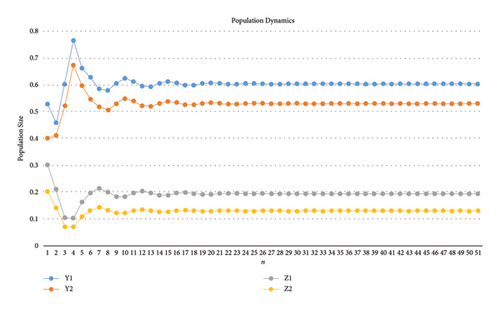
Example 1. First, we prove the local asymptotic stability of system (1). If we choose p1 = 3.09, p2 = 3, k1 = 2.51, k2 = 2.69, r11 = 2.99, r21 = 3, r12 = 0.01, r22 = 3.8, q1 = 1.121119, q2 = 1.121118, s11 = 3, s21 = 3, s12 = 0.593193 and s22 = 0.59319 with initial population (0.5274, 0.4, 0.3, 0.2), then the fixed point E(0.602943, 0.3333, 0.192216, 0.18601) of system (1) is locally asymptotically stable. The characteristic function and Jacobian matrix of system (1) for above parametric values are given by
Comparing above equation with (18), we have A = −1.494, B = 1.0681, C = −0.473691, and D = −0.100315. Moreover, the following conditions are satisfied:
Thus, all the conditions (20) are satisfied. For the above parametric values and n ∈ [1009, 1024], we have calculated the following numerical values of the population.
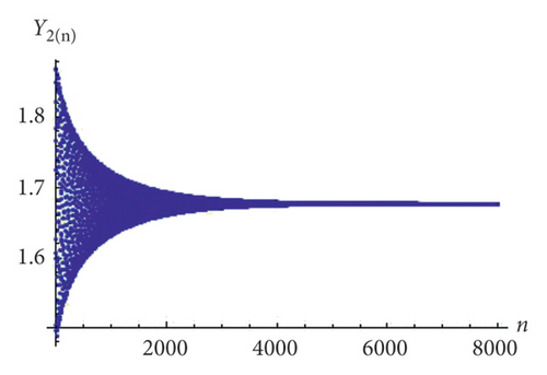
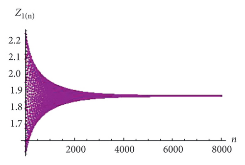
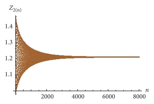
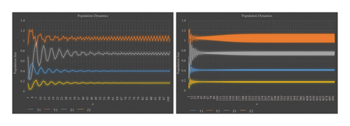
From the tabular values (Table 1), we see that whatever the value of n is taken, the behavior of system (1) is constant and is found in the closed neighborhood of E(0.641129, 0.333333, 0.160243, 0.163843). Therefore, the unique positive fixed point of system (1) is locally asymptotically stable. Furthermore, the initial dynamics and stability of the population can be evaluated from Figures 9, 10(a), 10(b), 10(c), and 10(d).
| n | Y1(n) | Y2(n) | Z1(n) | Z2(n) |
|---|---|---|---|---|
| 1009 | 0.602495 | 0.528722 | 0.192793 | 0.128659 |
| 1010 | 0.602495 | 0.528722 | 0.192793 | 0.128659 |
| 1011 | 0.602495 | 0.528722 | 0.192793 | 0.128659 |
| 1012 | 0.602495 | 0.528722 | 0.192793 | 0.128659 |
| 1013 | 0.602495 | 0.528722 | 0.192793 | 0.128659 |
| 1014 | 0.602495 | 0.528722 | 0.192793 | 0.128659 |
| 1015 | 0.602495 | 0.528722 | 0.192793 | 0.128659 |
| 1016 | 0.602495 | 0.528722 | 0.192793 | 0.128659 |
| 1017 | 0.602495 | 0.528722 | 0.192793 | 0.12866 |
| 1018 | 0.602495 | 0.528722 | 0.192793 | 0.12866 |
| 1019 | 0.602495 | 0.528722 | 0.192793 | 0.12866 |
| 1020 | 0.602495 | 0.528722 | 0.192793 | 0.12866 |
| 1021 | 0.602495 | 0.528722 | 0.192793 | 0.12866 |
| 1022 | 0.602495 | 0.528722 | 0.192793 | 0.12866 |
| 1023 | 0.602495 | 0.528722 | 0.192793 | 0.12866 |
| 1024 | 0.602495 | 0.528722 | 0.192793 | 0.12866 |

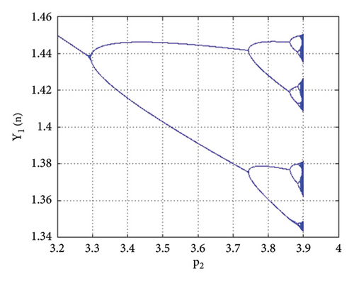
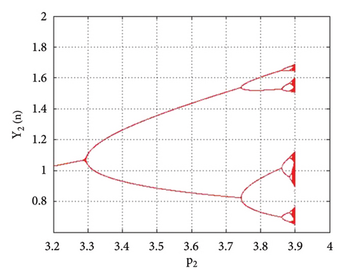
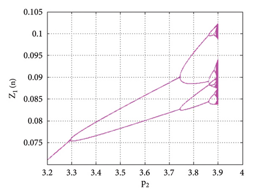
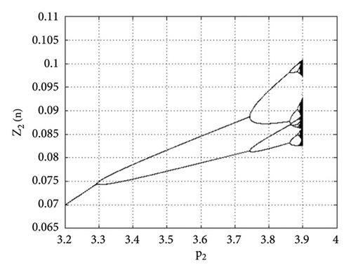
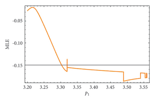
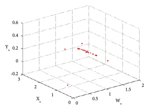
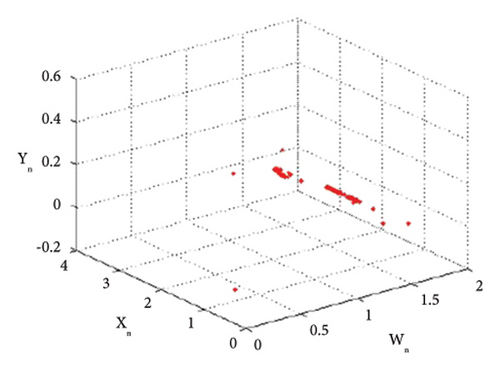
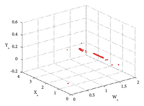
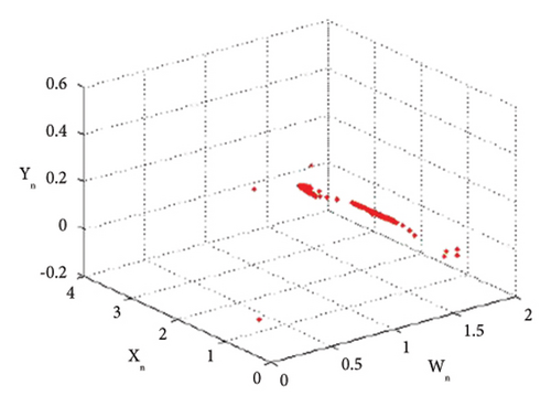
Example 2. In this example, we will study the period-doubling bifurcation occurring in the system. For this, we assume that the initial population is (0.23, 0.16, 0.1, 0.3), and the remaining parameters have the following values: p1 = 2.8, k1 = 1.1, k2 = 1.9, r11 = 2.1, r21 = 0.6, r12 = 0.8, r22 = 2.9, q1 = 1.1000099, q2 = 1.1, s11 = 1.200007, s21 = 1.2, s12 = 0.35, s22 = 0.35, p2 ∈ (3.2, 4). Then, the period-doubling bifurcation occurs at the unique positive fixed point (16) of system (1) when the intrinsic population dynamics of the prey p2 exceed 3.256672813598711. The bifurcation diagrams and MLE of system (1) are given in Figures 11(a), 11(b), 11(c), 11(d), and 11(e). The phase portraits are given in Figures 12(a), 12(b), 12(c), and 12(d). Thus, for p2 = 3.3 and above selected parametric values, the unique positive fixed point E(1.41429, 1.15102, 0.008731, 0.519939) is unstable. The Jacobian matrix and characteristic equation for p1 = 2.8, k1 = 1.1, k2 = 1.9, r11 = 2.1, r21 = 0.6, r12 = 0.8, r22 = 2.9, q1 = 1.1000099, q2 = 1.1, s11 = 1.200007, s21 = 1.2, s12 = 0.35, s22 = 0.35, p2 = 3.256672813598711 are as follows:
If A = −0.257347, B = −1.38302, C = 0.488477, and D = 0.151894, then we have the following conditions of period-doubling bifurcation from Lemma 11.
From tabular data in Table 2, we have noticed that the rapid dynamical fluctuation in population causes bifurcation in system (1).
Thus, all the conditions of the period-doubling bifurcation are satisfied. For a more detailed study, we find the population values of system (1) at the values of parameters selected above. The population values are listed in Table 2.
| n | Y1(n) | Y2(n) | Z1(n) | Z2(n) |
|---|---|---|---|---|
| 965 | 1.4459 | 0.9609 | 0.04989 | 0.14965 |
| 966 | 1.4241 | 1.2008 | 0.04847 | 0.14538 |
| 967 | 1.4459 | 0.9609 | 0.04989 | 0.14965 |
| 968 | 1.4241 | 1.2008 | 0.04847 | 0.14538 |
| 969 | 1.4459 | 0.9609 | 0.04989 | 0.14965 |
| 970 | 1.4241 | 1.2008 | 0.04847 | 0.14538 |
| 971 | 1.4459 | 0.9609 | 0.04989 | 0.14965 |
| 972 | 1.4241 | 1.2008 | 0.04847 | 0.14538 |
| 973 | 1.4459 | 0.9609 | 0.04989 | 0.14965 |
| 974 | 1.4241 | 1.2008 | 0.04847 | 0.14538 |
| 975 | 1.4459 | 0.9609 | 0.04989 | 0.14965 |
| 976 | 1.4241 | 1.2008 | 0.04847 | 0.14538 |
| 977 | 1.4459 | 0.9609 | 0.04989 | 0.14965 |
| 978 | 1.4241 | 1.2008 | 0.04847 | 0.14538 |
| 979 | 1.4459 | 0.9609 | 0.04989 | 0.14965 |
| 980 | 1.4241 | 1.2008 | 0.04847 | 0.14538 |
| 981 | 1.4459 | 0.9609 | 0.04989 | 0.14965 |
| 982 | 1.4241 | 1.2008 | 0.04847 | 0.14538 |
| 983 | 1.4459 | 0.96097 | 0.04989 | 0.14965 |
| 984 | 1.4241 | 1.20088 | 0.04847 | 0.14538 |
| 985 | 1.4459 | 0.96097 | 0.04989 | 0.14965 |
| 986 | 1.4241 | 1.20088 | 0.04847 | 0.14538 |
| 987 | 1.4459 | 0.96097 | 0.04989 | 0.14965 |
| 988 | 1.4241 | 1.20088 | 0.04847 | 0.14538 |
| 989 | 1.4459 | 0.96097 | 0.04989 | 0.14965 |
| 990 | 1.4241 | 1.20088 | 0.04847 | 0.14538 |
| 991 | 1.4459 | 0.96097 | 0.04989 | 0.14965 |
| 992 | 1.4241 | 1.20088 | 0.04847 | 0.14538 |
| 993 | 1.4459 | 0.96097 | 0.04989 | 0.14965 |
| 994 | 1.4241 | 1.20088 | 0.04847 | 0.14538 |
| 995 | 1.4459 | 0.96097 | 0.04989 | 0.14965 |
| 996 | 1.4241 | 1.20088 | 0.04847 | 0.14538 |
| 997 | 1.4459 | 0.96097 | 0.04989 | 0.14965 |
| 998 | 1.4241 | 1.20088 | 0.04847 | 0.14538 |
| 999 | 1.4459 | 0.96097 | 0.04989 | 0.14965 |
| 1000 | 1.4241 | 1.20088 | 0.04847 | 0.14538 |
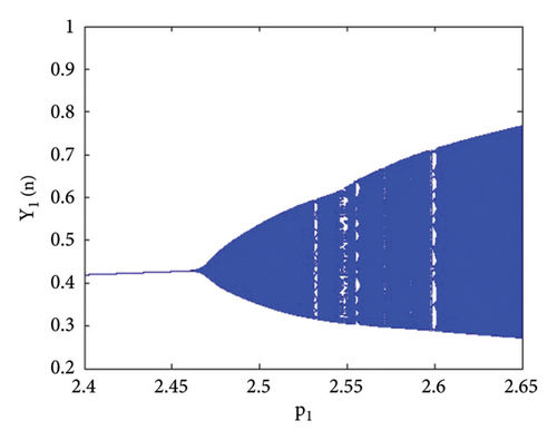
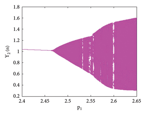
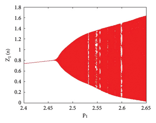
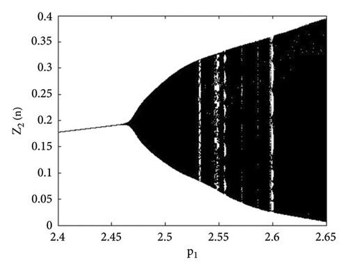
Example 3. Let us have p2 = 3.8, k1 = 2.2, k2 = 2.2, r11 = 0.6, r21 = 0.6, r12 = 0.2, r22 = 0.4, q1 = 1.9000042, q2 = 1.9, s11 = 3.200009, s21 = 3.2, s12 = 1.5, s22 = 1.5 with initial population (0.267, 0.938, 0.685, 0.165) and the bifurcation parameter p1 ∈ (2.4, 2.65). Then, the unique positive fixed point (16) of system (1) E(0.467, 0.938, 0.0163, 1.818) undergoes Hopf bifurcation. The bifurcation arises at p1 = 2.450640769328435. These parametric values satisfy all the conditions of Lemma 11. Therefore, Hopf bifurcation emerges for the abovementioned parametric values. The Jacobian matrix evaluated at the parametric values p2 = 3.8, k1 = 2.2, k2 = 2.2, r11 = 0.6, r21 = 0.6, r12 = 0.2, r22 = 0.4, q1 = 1.9000042, q2 = 1.9, s11 = 3.200009, s21 = 3.2, s12 = 1.5, s22 = 1.5, and p1 = 2.450640769328435 is given by
The characteristic function is
The spectrum of the above characteristic function is SExample2 = {λ1 = 0.672385, λ2 = 0.99999991337, and λ3,4 = 0.291304 ± 0.956631ı}, with |λ3,4| = 1 and |λ1,2| ≠ 1.
Moreover, all the conditions of Hopf bifurcation given in Lemma 11 are satisfied:
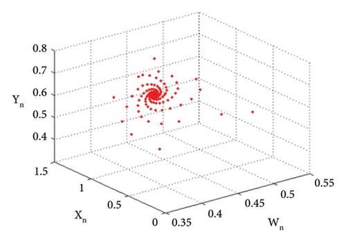
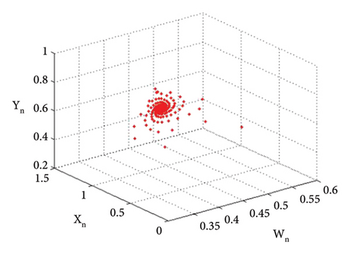
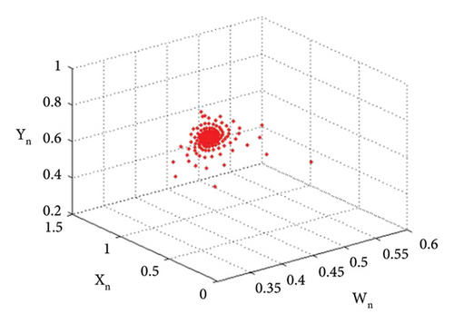
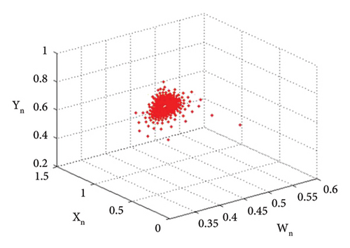
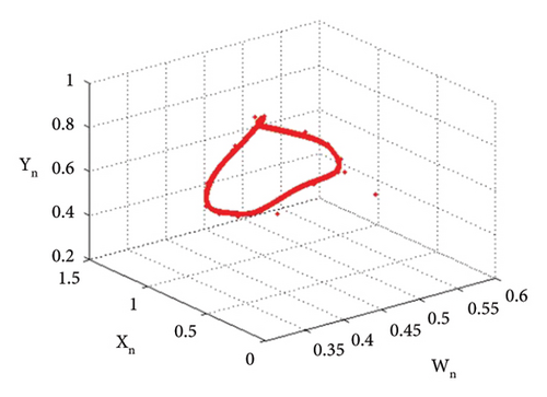
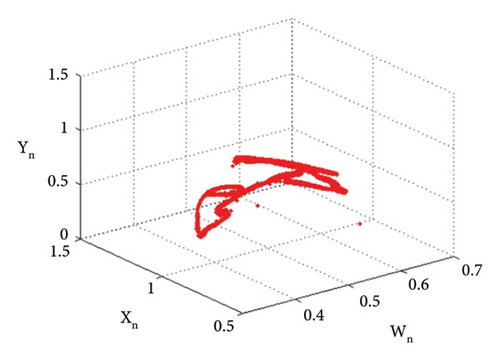
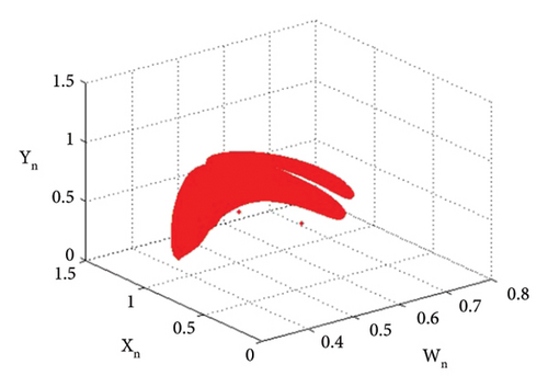
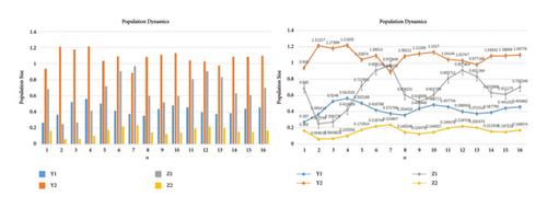
The bifurcation diagrams, the maximum Lyapunov exponent (MLE), and the phase plots of system (1) for the parametric values p2 = 3.8, k1 = 2.2, k2 = 2.2, r11 = 0.6, r21 = 0.6, r12 = 0.2, q1 = 1.9000042, r22 = 0.4, q2 = 1.9, s21 = 3.2, s11 = 3.200009, s12 = 1.5, s22 = 1.5, p1 ∈ (2.41, 2.65) with initial conditions (0.267, 0.938, 0.685, 0.165) are depicted in Figures 13(a), 13(b), 13(c), 13(d), 13(e), 14(a), 14(b), 14(c), 14(d), 14(e), 14(f), 14(g), and 14(h). The population dynamics for the above parametric values when n ∈ [0, 15] are given in Table 3.
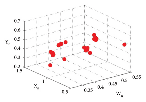
The graphical analysis for the above tabular population dynamics is given in Figure 15.


| n | Y1(n) | Y2(n) | Z1(n) | Z2(n) |
|---|---|---|---|---|
| 0 | 0.267 | 0.938 | 0.685 | 0.165 |
| 1 | 0.365416 | 1.21227 | 0.247558 | 0.059631 |
| 2 | 0.5246 | 1.17899 | 0.269278 | 0.0648629 |
| 3 | 0.562025 | 1.21635 | 0.416626 | 0.100356 |
| 4 | 0.502168 | 1.03874 | 0.717851 | 0.172914 |
| 5 | 0.416768 | 1.09013 | 0.908116 | 0.218744 |
| 6 | 0.372796 | 0.886372 | 0.970649 | 0.233807 |
| 7 | 0.354416 | 1.08211 | 0.604231 | 0.145546 |
| 8 | 0.435449 | 1.11209 | 0.518006 | 0.124776 |
| 9 | 0.481717 | 1.1317 | 0.601704 | 0.144937 |
| 10 | 0.457734 | 1.04144 | 0.805712 | 0.194078 |
| 12 | 0.372514 | 0.977168 | 0.832264 | 0.200474 |
| 13 | 0.387793 | 1.08542 | 0.630686 | 0.151918 |
| 14 | 0.441332 | 1.08899 | 0.611173 | 0.147218 |
| 15 | 0.455862 | 1.09779 | 0.700246 | 0.168674 |
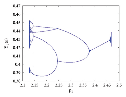
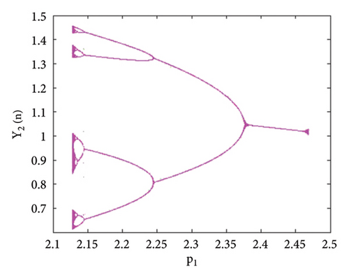
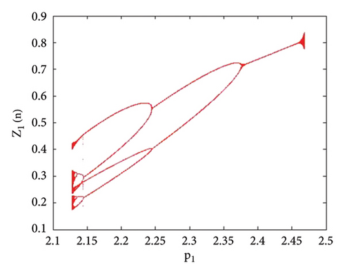
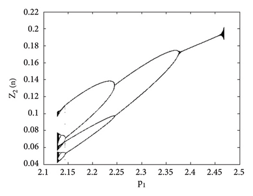
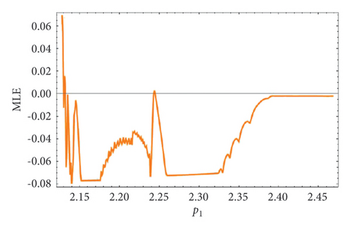
Example 4. Let us have the same parametric values as given in Example 3: p2 = 3.8, k1 = 2.2, k2 = 2.2, r11 = 0.6, r21 = 0.6, r12 = 0.2, r22 = 0.4, q1 = 1.9000042, q2 = 1.9, s11 = 3.200009, s21 = 3.2, s12 = 1.5, s22 = 1.5 with the assumed initial population (0.267, 0.938, 0.685, 0.165) and the bifurcation parameter p1 ∈ (2.128, 2.468). Then fixed point (16) of system (1) E(0.467, 0.938, 0.0163, 1.818) undergoes backward period-doubling bifurcation when we choose the intrinsic population dynamics p1 of prey as a bifurcation parameter. The system bifurcates if the intrinsic population dynamics p1 exceed 2.3951044645684285. The phase plots for different bifurcation parameter values p1 are given in Figures 16(a), 16(b), 16(c), 16(d), 16(e), and 16(f). The Jacobian matrix at the listed parametric values is given below:
The characteristic polynomial is
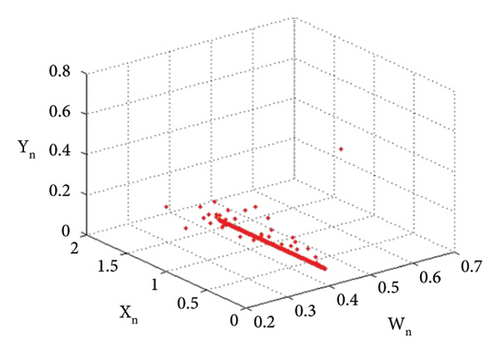
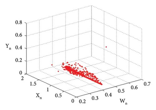
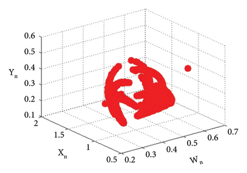
Thus, all the conditions of the period-doubling bifurcation are satisfied. The statistical data demonstrated for various time steps provide an overview of the real trajectories of the populations under the specified parameter values. These data points show population expansion, decline, or fluctuation patterns, allowing us to see how populations vary over time. We can better understand ecosystems and make well-informed decisions and model validation by using statistical data in ecological studies to describe complicated population patterns and identify trends, linkages, and major drivers. We have the following numerical values (Table 4) of population.
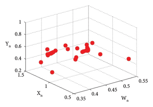
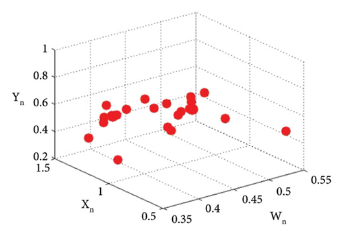
The graphical analysis of the statistical data is given in Figure 18.
| n | Y1(n) | Y2(n) | Z1(n) | Z2(n) |
|---|---|---|---|---|
| 1 | 0.365416 | 1.21227 | 0.247558 | 0.059631 |
| 2 | 0.5246 | 1.17899 | 0.269278 | 0.0648629 |
| 3 | 0.562025 | 1.21635 | 0.416626 | 0.100356 |
| 4 | 0.502168 | 1.03874 | 0.717851 | 0.172914 |
| 5 | 0.416768 | 1.09013 | 0.908116 | 0.218744 |
| 6 | 0.372796 | 0.886372 | 0.970649 | 0.233807 |
| 7 | 0.354416 | 1.08211 | 0.604231 | 0.145546 |
| 8 | 0.435449 | 1.11209 | 0.518006 | 0.124776 |
| 9 | 0.481717 | 1.1317 | 0.601704 | 0.144937 |
| 10 | 0.457734 | 1.04144 | 0.805712 | 0.194078 |
| 11 | 0.398568 | 1.02747 | 0.907964 | 0.218708 |
| 12 | 0.372514 | 0.977168 | 0.832264 | 0.200474 |
| 13 | 0.387793 | 1.08542 | 0.630686 | 0.151918 |
| 14 | 0.441332 | 1.08899 | 0.611173 | 0.147218 |
| 15 | 0.455862 | 1.09779 | 0.700246 | 0.168674 |
Example 5. Let us have the parametric values as p2 = 3.8, k1 = 2.2, k2 = 2.2, r11 = 0.6, r21 = 0.6, r12 = 0.2, r22 = 0.4, q1 = 1.9000042, q2 = 1.9, s11 = 3.200009, s21 = 3.2, s12 = 1.5, s22 = 1.5, and p1 ∈ (2.128, 2.6) with initial conditions (0.267, 0.938, 0.685, 0.165).
Then the positive fixed point (16) E(0.467, 0.938, 0.0163, 1.818) of system (1) experiences backward period-doubling and Hopf bifurcation. If we choose p1 as a bifurcation parameter, then the fixed point of system (1) loses its stability at p1 = 2.3951044645684285 and undergoes period-doubling bifurcation. But for p1 = 2.450640769328435, system (1) experiences Hopf bifurcation. All the conditions of period-doubling and Hopf bifurcation are satisfied. Further details related to the backward period-doubling bifurcation are given in Example 5.3, and details related to Hopf bifurcation will be discussed in Example 5.4. Figure 19 gives the bifurcation diagrams and maximum Lyapunov exponent.

6. Bi-Parameter Analysis
In this section, we will use two parameter plots to confirm the periodic behavior of system (1). We use different parameter values to construct other plots to check the periodic behavior of the system. When we better understand the cycles of predator and prey populations, we can better predict and control interactions between species in the field. Also, the periodicity will confirm the coexistence of the population. In domains like ecosystem conservation and resource management, periodicity is essential. To build more accurate and reliable ecological models, it can be helpful to understand the fundamental processes that support population dynamics by analyzing the periodic characteristics of these relationships. Here, we use the intrinsic population dynamics of the prey p1 and p2 to study the periodic circles between these populations. Similarly, one can also use other parameters to analyze the population dynamics.
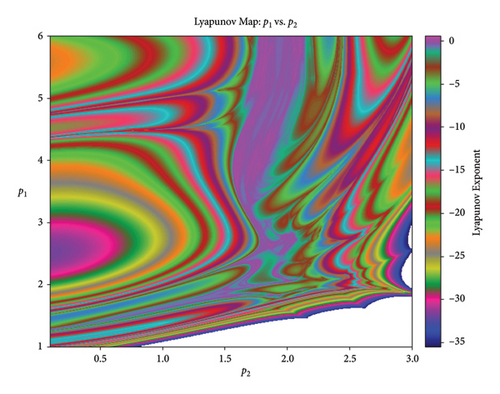
Here, we have used three different periodic plots to represent the various aspects of the populations. The first plot is the Lyapunov exponent between these two parameters (see Figure 20). We have employed the following parameter values for this: k1 = 1.2, k2 = 0.2, r11 = 0.6, r12 = 1.6, r21 = 0.5, r22 = 0.4, s11 = 1.29, s12 = 1.5, s21 = 1.2, s22 = 1.5, q1 = 2.1, q2 = 1.9 with parameter space p1 × p2 ∈ [0.01, 3.0] × [0.01, 3.0]. Here, we choose (0.067, 0.138, 0.285, 0.265) as the initial population. We have seen the negative values in this plot. The negative values of the Lyapunov exponent represent the periodicity of the model. This means the predator-prey population is stable and can sustain itself over time. Even slight modifications to the system’s initial conditions will eventually result in a stable equilibrium state, where the populations of prey and predators oscillate.
In the second plot, we have drawn the basin of attraction between the same two parameters. A basin of attraction is a region of phase space that attracts trajectories toward a particular equilibrium state. Here, we fix the following values of the parameters: k1 = 0.2, k2 = 0.3, r11 = 0.2, r12 = 0.3, r21 = 0.4, r22 = 0.5, s11 = 0.6, s12 = 0.7, s21 = 0.8, s22 = 0.9, q1 = 0.01, q2 = 0.03 with parameter space p1 × p2 ∈ [0, 2] × [0, 2] and initial population (0.2, 0.3, 0.2, 0.1).
Figure 21 shows different periods of basins of attraction. This indicates the other possible equilibrium states the system can converge toward, depending on parameter values.
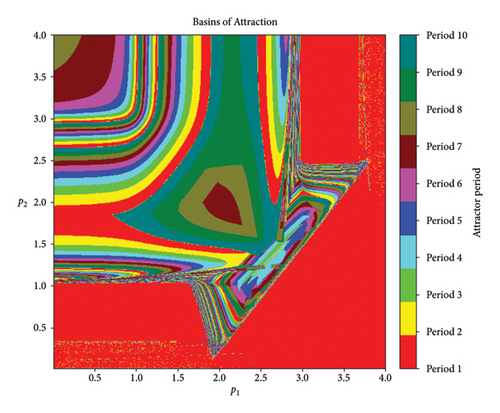
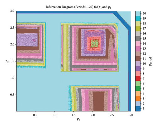
Figure 22 is the periodic plot with twenty different periods. For this plot, we use the following values of parameters: k1 = 1.8, k2 = 1.6, r11 = 0.3, r12 = 0.4, r21 = 0.5, r22 = 0.6, s11 = 0.8, s12 = 0.9, s21 = 0.8, s22 = 0.6, q1 = 0.7, q2 = 0.8 in the space p1 × p2 = [0.1, 3.0] × [0.1, 3.0] with the initial conditions (0.15, 0.14, 0.13, 0.12). Through this plot, we confirm the cyclical nature of the prey-predator population. This plot confirms the rise and fall of predator and prey populations in a predictable manner. Through all these plots, we confirm the stability of the system, the different equilibrium states, and the coexistence of the population. Thus, external forces like changes in the environment or human interaction do not dramatically alter the system’s dynamics; the system’s ability to sustain itself over an extended period is suggested by its periodic behavior.
7. Dynamics of Chaos in the Four-Dimensional Model
Li and Yorke presented the first formal definition of discrete chaos [51], establishing easy criteria for chaos in one-dimensional dynamical systems. The result was then extended to higher-dimensional dynamical systems by Marotto [52] and Marotto [53]. However, the original Marotto theorem contained a mistake in its condition, which Shi and Chen [54] corrected and revised. We will apply this theory to our system (3) using these criteria to verify that chaos exists in our model. In this section, we discuss the chaos under the influence of bifurcation.
Lemma 16 (see [55].)Let a continuous map in the interval . Suppose that a point exists that satisfies
- (1)
For every ,
(52) -
and
(53) - (2)
For every and periodic point with μ1 ≠ μ2,
(54) -
When the one-dimensional dynamical system ηm+1 = ξ(ηm) meets the above requirements, it is considered chaotic according to Li and Yorke. Marotto extended Li and Yorke’s research to the n-dimension by proving the subsequent theorem.
Theorem 17 (see [54]–[56].)Consider the subsequent n-dimensional discrete system.
- (i)
At the fixed point η, all of the eigenvalues of the Jacobian Dξ(η) of map (7.1) have euclidean norms greater than one.
- (ii)
There exist some ϵ > 1 and γ > 0, such that for all ,
Shi and Chen demonstrated that the original Marotto theorem included a conditional error that has been fixed. The revised theorem is provided as follows.
Theorem 18 (see [55].)Consider the subsequent n-dimensional discrete system.
- (i)
In a neighborhood of η∗, ξ is continuously differentiable, and all of the eigenvalues Dξ(η∗) have absolute values greater than one. This implies the existence of a positive constant γ and a euclidean norm, such that ξ is expanding in in the euclidean norm, and
- (ii)
η∗ is a snap-back repeller of ξ with ξm(η0) = η∗ for some , η0 ≠ η∗ and some positive integer m. Furthermore, ξ is continuously differentiable in some neighborhoods of η0, η1, η2, ηm−1, respectively, and det[Dξ(ηj)] ≠ 0 for 0 ≤ j ≤ m − 1, where ηj = ξ(ηj−1). Then, every Marotto theorem finding is true.
Lemma 19. If αg = (q1 + 1)k2 + s12/s12, αh = (q2 + 1)k2 + s22/s22, and p2 > 1, then system (1) is chaotic when |p2| > max{3, αg, αh} and |p1| > 1.
Proof. Let be the fixed point of (1); then it can be written as η∗ = ξ(η∗). If Y1 = η1, Y2 = η2, Z1 = η3, and Z2 = η4, then ξ(η) is represented by system (1). Also, ξ(η) is continuously differentiable in for some γ > 0. At the fixed point η∗, we have calculated the following Jacobian matrix:
The latent roots of the D(ξ(η∗)) are given as λ1 = p1, λ2 = 2 − p2, λ3 = (p2 − 1)s12/k2 − q1, and λ4 = (p2 − 1)s22/k2 − q2.
|λ1,2,3,4| > 1 holds if
Thus, according to the first condition of Theorem 17, the fixed point η∗ is an expanding fixed point of ξ of system (1) since all the eigenvalues of D(ξ(η∗)) are greater than one. Consequently, ϕ is expanding in , provided that γ > 0 and the Euclidean norm ‖.‖ exist. That is to imply that we have ‖ξ(ζ) − ξ(η)‖ > ϵ‖ζ − η‖, for any two distinct points , where ϵ > 1 and ζ, η are sufficiently close to η∗. Since ξ(ζ) − ξ(η) = Dξ(η)(ζ − η) + β, therefore ‖β‖/‖ζ − η‖⟶0 as ‖ζ − η‖⟶0. Specially, we have ‖ξ(η) − ξ(η∗)‖ = ‖Dξ(η∗)(η − η∗) + β‖, with the euclidean norm of a real matrices of order (m, n). Since ξ(η) is continuously differentiable, Dξ(η∗) is expanding for . The norm of Dξ(η∗) is given by
Consequently, both the conditions of Theorem 17 are satisfied. According to Theorem 17, for snap-back repeller, we need to find one point , such that ζ ≠ η∗, ξn(ζ) = η∗, and det[Dξn(ζ)] ≠ 0, for some positive integer n. We have
From above systems of (61) and (62), we have collected a solution (0, 1/k2, 0, 0) such that and ζ ≠ η∗. Now, an operator ξ2 has been constructed to map the point ζ = (Y1, Y2, Z1, Z2) to the fixed point . After two iterations if there are solutions different from ζ∗ for systems (61) and (62), then we can also calculate the solutions for the system (1) that differ from ζ∗. So, we also can calculate the solutions for system (1) that differ from ζ∗.
The solution ζ = (0, p2 − 1/k2, 0, 0) is now accepted, with ζ ≠ η∗ and ξ2(ζ) = η∗. Following is the computation of the Jacobian matrix of ξ2 at ζ:
As a result, each condition of Theorem 17 is satisfied.
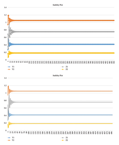
The unique positive fixed point of the controlled system (65) is locally asymptotically stable if roots of the characteristic polynomial of (66) lie in an open disk. We have the stability plot for system (66) in Figure 23.
8. Conclusion
In this paper, we analyzed the dynamic behavior of the four-dimensional predator-prey model. We calculate eleven fixed points that are also ecologically valid. Prey populations can survive without predators because the survival of prey does not depend on predators E1, E2, and E3. The fixed points E4, E5, E6, E7, E8, and E9 represent that the population of both predators can stay in the presence of one or both prey because prey will be available for the predator as a source of food. The population of both predators can survive with both prey E10. Still, if both prey populations are depleted, the population of both predators will die out due to reduced food availability E0. We have calculated the parametric conditions for the stability of all fixed points and drawn graphs to determine the latent roots’ behavior. Mainly, we study the existence of biologically feasible solutions to the positive fixed points. We confirm that our ecological model can sustain itself over time through detailed, novel periodic plots. The slight modifications to the system’s initial conditions will eventually result in a stable equilibrium state, where prey and predator populations oscillate. Through the basin of the attraction plot, we provide all possible convergent equilibrium states. Thus, we confirm the stability of the model, the equilibrium states, and the coexistence of the populations in terms of periodic plots. In addition, we have seen that when the intrinsic dynamics of the population exceed a certain threshold, the system bifurcates. This particular range of inherent population dynamics depends on the values of other biological parameters and the initial population. Moreover, we proved that the instability of the model resulted in Neimark–Sacker and period-doubling bifurcation. We used bifurcation theory to verify these two types of bifurcation and graphical results to find the direction of bifurcation. The observed bifurcation behavior in our model can be understood as the ecological system responding sensitively to variations in the intrinsic growth rates of prey populations (p1 and p2). These bifurcations represent shifts in the qualitative behavior of the predator-prey dynamics, providing insights into the system’s stability and the potential for complex, oscillatory patterns in response to changes in vital ecological parameters. These findings contribute to understanding how simple ecological models can give rise to complex dynamics and highlight the importance of considering nonlinear interactions in studying population ecology. The computer simulation of the maximum Lyapunov exponents demonstrates that the model exhibits chaotic behavior. Numerical simulations are provided to display the outcomes of the theory. From numerical examples, we proved both types of bifurcation occurring in the system for specific values of the parameters. From the tabular data, we have confirmed that the uncertainty of population growth is due to bifurcation. We constructed tables to show the rate of change in the populations for these selected parameters’ values. These simulation findings show chaotic long-term behavior over an extensive range of parameters. Thus, we proved the bifurcation in the system both by bifurcation theory and tabular data. We employ Marotto’s theory to confirm the existence of chaos in the ecological mode. Finally, we use a hybrid control feedback methodology to control the chaos.
Additional Points
Future Work on Updated Model. In the future, we will update this model and provide interesting results related to this model.
Ethical Approval
All procedures followed were by ethical standards.
Conflicts of Interest
The authors declare that there are no conflicts of interest.
Authors’ Contributions
All authors contributed equally.
Acknowledgments
This work was supported by the Deanship of Scientific Research, Vice Presidency for Graduate Studies and Scientific Research, King Faisal University, Saudi Arabia (grant no. 5938).
Open Research
Data Availability
No data were used to support this study.


