Assessing the Impact of Climate Change on Agricultural Water Management in Mainland Southeast Asia
Abstract
This study aims to address an assessment of climate change’s impact on agricultural water management in mainland Southeast Asia (MSEA). We used several agroclimatic indices, such as consecutive dry days (CDDs), maximum number of consecutive wet days (CWDs), consecutive summer days (CSUs), cold spell duration index (CDSIs), and warm and wet days (WWs), based on the Geophysical Fluid Dynamics Laboratory Earth System Model to characterize the effect of climate on crop water need (CWN) in MSEA. The climate model shows monthly precipitation and temperature patterns with acceptable accuracy but with an underestimation of precipitation and a warm bias in temperature. CDDs show a significant increase in aridity and drought occurrences, particularly in northern Myanmar, Laos, Vietnam, and northern Thailand, across different representative concentration pathways. CSUs have been seen to have a substantial influence on the region’s agricultural economy. The CDSIs, on the other hand, show a decrease in the duration of cold spells, indicating the existence of milder climatic conditions that could potentially affect crop growth. The CWDs show a decreasing trend in most of the multiple regions in Thailand, Laos, Vietnam, Cambodia, and Malaysia. Though the WW index shows more wet days, this does not immediately imply improved crop growth; rather, it highlights possible changes in water availability that could affect agricultural practices. While negative CWNs in the dry season months like March and November suggest possible water shortages, which pose risks to agriculture and food security in Myanmar, northern and eastern Thailand, and Cambodia, especially at the end of the century, increases in CWNs during the rainy season correspond with anticipated higher water demands for agriculture.
1. Introduction
Climate change is clearly having an influence on mainland Southeast Asia (MSEA), an area renowned for its varied topography and agricultural importance [1, 2]. These elements bring with them a plethora of intricate problems, especially because agriculture, which provides a significant amount of MSEA’s income and food security, is so important [3]. MSEA has a predominantly monsoonal climate with considerable temperature and precipitation variability. Precipitation totals vary yearly from about 1,200 mm in the drier core parts to over 3,000 mm along the coast [3]. Temperature swings are also noticeable; multiyear seasonal averages range from 22°C in the colder months to 30°C at the height of the hot season [3]. These climatic factors are critical because they have an immediate impact on water resource management and agricultural productivity. Extreme weather occurrences in MSEA become more intense when climate change manifests itself in significant temperature swings and changes in precipitation patterns [4]. Variations in precipitation leading to extended periods of excessive rainfall, which pose serious concerns, such as waterlogging and erosion, especially in agriculturally dependent regions, are making these changes more and more apparent [5]. Moreover, the complex system of linked rivers and watersheds in MSEA, which is necessary for irrigation and crop production, makes the area more susceptible to the effects of climate change [6]. The need to know and adjust to shifting climatic conditions to protect and maybe improve agricultural output and general regional stability is highlighted by the reliance on these water resources.
While significant progress has been made in understanding the climate changes occurring in MSEA, concerns are mounting regarding the repercussions for the agricultural sector. Challenges loom large, particularly in the realm of sustaining food production amidst the anticipated rise in drought frequency, prolonged arid spells, and soaring temperatures [7]. Changes in agroclimatic indices, including an increase in consecutive dry days (CSUs) and warm and wet days (WWs), raise pertinent questions about crop suitability and effective water resource management [8]. Agriculture serves as the linchpin of the region’s economy, providing sustenance and employment to a substantial portion of its populace. The ramifications of an agricultural crisis are far-reaching, as it not only imperils food security but also bears broader societal consequences. Given the intricate interplay between climate change and agriculture in MSEA, a comprehensive, context-specific assessment is imperative to better comprehend the potential challenges and opportunities associated with adapting to a changing environment.
Prior studies have explored the relationship between global warming, particularly the severity of drought, on agriculture and water resources. Dai [8] conducted a comprehensive review highlighting the implications of global warming on drought occurrences, shedding light on the increasing frequency and severity of droughts influenced by climate change. Lobell and Field [9] focused on the critical connection between climate change and global crop yields, investigating how recent warming trends impact crop production and its implications for food security. Porter and Semenov [10] delved into how crops respond to climatic variations, emphasizing the significance of understanding the interplay between agriculture and weather conditions. Hatfield et al. [11] collectively underscored the urgent need to address the complex relationship between climate change and agriculture, emphasizing the importance of proactive adaptation measures and resilient agricultural practices.
In this research, our study seeks to address an assessment of the impact of climate change on agricultural water management in MSEA. This approach aims to offer a more nuanced, region-specific understanding of the challenges and opportunities in agricultural water management, thereby guiding decision-makers toward more effective climate adaptation and mitigation strategies. Our study focuses on specific agroclimatic indices—consecutive dry days (CDDs), CSUs, cold spell duration index (CDSI), consecutive wet days (CWDs), and WWs that directly influence crop water requirements. By delving into the intricate relationships between these indices and crop water needs (CWNs), we endeavor to provide a holistic comprehension of the challenges and opportunities that climate change presents to agriculture in MSEA. Furthermore, our study encompasses a nuanced examination of multiple representative concentration pathways (RCPs), including RCP2.6, RCP4.5, RCP6.0, and RCP8.5, to encompass a wide spectrum of potential climate futures. This approach allows us to assess a broad range of climate scenarios, yielding valuable insights for the development of adaptation and mitigation strategies.
2. Methodology
The purpose of this study was to examine the impact of climate change on agricultural water management in MSEA during 1981–2099. We used the data from the Geophysical Fluid Dynamics Laboratory Earth System Model (GFDL ESM) under scenarios from the Coupled Model Intercomparison Project Phase 5 (CMIP5). The future projection covers a wide range of projected climate change, with an emphasis on RCP2.6, RCP4.5, RCP6.0, and RCP8.5 [12]. These scenarios, which are particularly important for water management and agricultural planning, offer insights into various degrees of climate mitigation measures and their effects on regional climates. The study covers a standard 30-year climatological period in climate impact research, which typically encompasses both mid-century and end-of-century time periods. Four separate periods comprised the analysis: 1981–2010 (the baseline period), 2011–2040, 2041–2070, and 2071–2099. The temperature data from GFDL ESM was utilized as an input parameter for predicting CWN.
2.1. Study Area
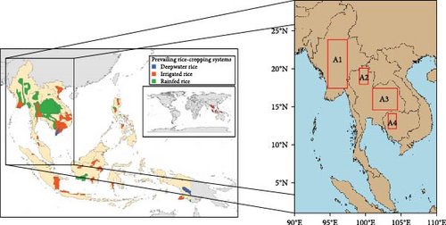
The study area encompasses six different countries within MSEA, namely Cambodia, Laos, Myanmar, Thailand, Vietnam, and Peninsular Malaysia. The MSEA region has a vast landmass spanning over 2 million square kilometers. Cropland and forest occupy the mainland areas, accounting for 38% and 41.5% of the total, respectively (Figure 1). According to the European Space Agency, rainfed-based croplands constitute the predominant proportion, amounting to approximately 85% [13, 14]. In this study, we selected four areas in difference countries including Myanmar (latitude 17°N to 24°N and longitude 94.5°E to 97.5°E) namely “A1”, Thailand (Northern: latitude 18°N to 20°N and longitude 99°E to 100.5°E, namely “A2”, Northeastern: latitude 14.5°N to 17°N and longitude 101°E to 104.5°E, namely “A3”)), and Cambodia (latitude 12.5°N to 14°N and longitude 105.5°E to 104°E, namely “A4”) (Figure 1).
Under tropical conditions and with adequate irrigation, two to three rice harvests per year are conceivable [1]. The differences in growing seasons and crop calendars are determined by the cultivar being grown. Rice is the only crop that thrives in wetland conditions, according to Bouman [15]. Rice-growing environments can thus be classified into four basic agricultural systems based on criteria such as water regime, drainage, temperature, soil type, and terrain. The climatic conditions within the region exhibit considerable variation throughout different geographies and seasons, ultimately falling within the tropical monsoon climate classification. The dry season is characterized by minimal precipitation and elevated temperatures. The region experiences a monsoon environment, which gives rise to two distinct growing seasons: a dry season spanning from November to May and a rainy season occurring from June to December. Rice cultivation is predominantly practiced during both seasons.
2.2. Climate Data Used
This study derives the agroclimatic indices from the GFDL ESM [16], sourced from the Climate Data Store (CDS) (https://cds.climate.copernicus.eu/). Similar to the physical climate models developed by GFDL, it incorporates an atmospheric circulation model that relates to an oceanic circulation model. While Earth System Models (ESMs) are designed to include interacting biogeochemical processes, such as the carbon cycle. The atmospheric component of ESMs encompasses various physical aspects, including aerosols, cloud physics, and precipitation. This study utilizes a dataset that provides agroclimatic indicators to effectively assess the impact of climate change on agriculture on a global scale. Agroclimatic indicators serve as valuable tools for communicating climate variability and change in a manner that is relevant to the agricultural industry. The primary goal of this collection is to provide these indicators on a global scale in a readily accessible and practical format for subsequent study and application of agricultural impact models. We have derived the agroclimatic indicators for both historical and future time periods using the GFDL ESM datasets. The agroclimatic indicators were derived using the WFDEI (Watch Forcing Data methodology) [17] for the climatology study. The dataset contains a complete collection of 26 different indicators, each carefully chosen and shown at a spatial resolution of 0.5° × 0.5°, using a longitudinal and latitudinal grid.
To examine the performance of the principal factors of agroclimatic indices, such as temperature and precipitation, they were compared to the Global Land Data Assimilation System (GLDAS) version 2. The information of GLDAS was described in Rodell et al. [18]. This system’s primary goal is to absorb satellite and ground-based observational data outputs using sophisticated land surface modeling and data assimilation algorithms. The goal of this approach is to generate optimal representations of land surface states and fluxes. GLDAS sets itself apart with its uncoupled land surface modeling system, enabling the operation of multiple models simultaneously. Furthermore, GLDAS distinguishes itself through the incorporation of a significant amount of observation-based data, global coverage at a high resolution of 0.25°, and the capacity to provide findings in the near-real time of the present instant.
2.3. Agroclimatic Indices
This study examined the changing climate trends related to agriculture in MSEA using a variety of agroclimatic indices, as listed in Table 1, such as CDDs, CSUs, CDSI, CWDs, and WWs, among others. These indices were selected due to their direct relevance to agricultural productivity and water management. For example, protracted dry spells necessitate higher water supplementation to maintain crop health, and CDDs directly impact irrigation needs and crop stress levels. CSUs show how many days in a row the temperature is higher than a threshold that is particular to the crop. Overheating plants without sufficient water can accelerate crop maturation and reduce overall yield. CDSIs measure how long major cold episodes last, which can impact plant dormancy periods and are essential for growing temperate crops that need cooling for fruit set and growth. WWs show days with high temperatures and amounts of water, which can help some crops grow but also make pests and diseases more likely, so they need to be carefully managed and watched. CWDs, on the other hand, show days when it rains a lot, which changes the level of saturation in the soil and the risk of waterlogging, which can cause root diseases and less oxygen for plants.
| Full name | Abbreviation (unit) | Definition |
|---|---|---|
| Maximum number of consecutive dry days | CDDs (day) | The longest duration of consecutive days with a cumulative daily precipitation (RR) of less than 1 mm [19, 20, 21]. |
| Cold spell duration index | CSDIs (day) | The annual count of days exhibiting a minimum of 6 consecutive days in which the daily maximum temperature (TX) remains below the 10th percentile of the calendar day (TX10th). To determine the TX10th value for each day a statistical approach is employed. This involves utilizing a 5-day window centered on each corresponding day throughout the 1981–2010 period [22]. |
| Maximum number of consecutive wet days | CWDs (day) | The longest duration of consecutive days during which the cumulative sum of daily precipitation (RR), exceeds 1 mm [19]. |
| Warm and wet days | WWs (day) | Number of days every 10 days when the daily mean temperature (TG) is more than the calendar day 75th percentile (TG75th) and the sum of daily precipitation (RR) is greater than the wet day 75th percentile (RR75th). To determine the TG75th and RR75 for each day, a 5-day set centered on each analogous day from 1981 to 2010 is utilized to improve statistical reliability, and the data’s 75th percentile is used [23]. |
| Maximum number of consecutive summer days | CSUs (day) | The longest run of days in a row is when TX > 25°C, where TX has the highest temperature of the day. This indicator gives data on optimal growth for C4 crops (e.g., maize) or on drought stress. |
2.4. Evaluation of Model Performance
2.5. CWN
CWN is defined by Pidwrny [25] as the state of balance between water demand and supply in the context of irrigation management. It is a useful tool for planning agricultural productivity. CWNs are calculated by considering two variables: potential evapotranspiration (PET) and actual evapotranspiration (AET). PET is the process of evaporation and transpiration that is responsible for the removal of surface water from the atmosphere. The word “AET” refers to the amount of water lost from the Earth’s surface because of evaporation and transpiration working together.
3. Result and Discussion
3.1. Model Evaluation
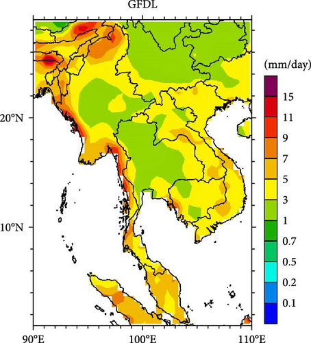
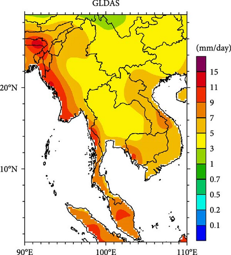
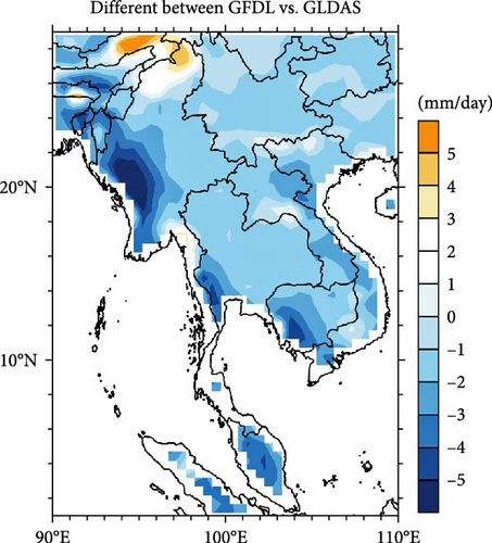
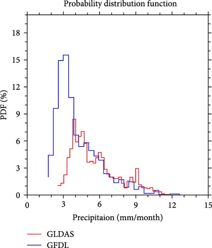
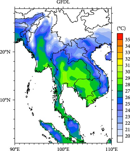
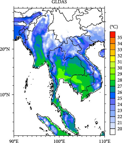
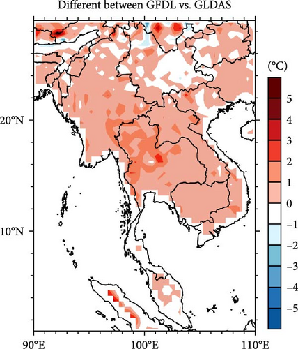
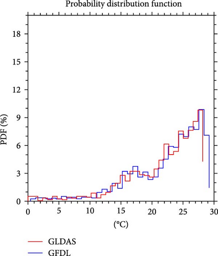
Figures 2 and 3 illustrate the validation procedure concerning the discrepancy observed in the monthly mean precipitation and temperature, notably within the temporal range of 1981–2010, as it is averaged between the GFDL model and the GLDAS datasets. Based on the GFDL model, it exhibits a tendency to underestimate precipitation when compared to GLDAS over the studied region. Additionally, the temperature model displays a generally warm bias throughout the whole area. The probability distribution function (PDF) demonstrates a significant similarity between the datasets obtained from the GFDL model and the GLDAS. Both datasets displayed precipitation levels ranging from 0 to 10 mm/month, along with temperatures falling within the range of 21 to 28°C. Nevertheless, it was noted that the GLDAS dataset exhibited a higher magnitude of precipitation, with an increase of 2–3 mm/month and temperatures ranging from 1 to 2°C. The statistical calculations on the comparison between the GFDL and GLDAS have been consolidated annually, covering the years 1981–2010, as presented in Table 2. The model demonstrates a significant ability to capture both variables, as indicated by the R-squared values of 0.50 and 0.98 for precipitation and temperature, respectively. The observed correlation coefficient between the variables was found to be 0.66 for precipitation and 0.99 for temperature. Additionally, the MBE showed values of −0.005 mm/month for precipitation and −0.005°C for temperature. The study recorded RMSE values of 2.08 and 0.53 for precipitation and temperature, respectively. While the SDR was 0.02 and 0.01 for precipitation and temperature, respectively.
| Variable | MBE | CC | R2 | RMSE | SDR |
|---|---|---|---|---|---|
| Temperature | 0.0 (°C) | 0.99 | 0.98 | 0.53 (°C) | 0.01 (°C) |
| Precipitation | 0.0 (mm/month) | 0.66 | 0.50 | 2.08 (mm/month) | 0.02 (mm/month) |
The GFDL model frequently exhibits a tendency to underestimate precipitation in comparison to the GLDAS model within the designated study area. The potential cause for the observed disparity of 2–3 mm/month in favor of GLDAS could be attributed to various causes. The utilization of parameterization strategies within the GFDL model is of utmost importance in accurately simulating precipitation. Discrepancies may arise due to variations in cloud microphysics, convection, and other related processes [29]. The portrayal of local-scale elements and processes contributing to precipitation patterns can be strongly influenced by spatial resolution. Lower resolutions may not adequately represent fine-scale meteorological phenomena or orographic influences [30]. The GLDAS model incorporates observational data into its modeling framework, hence enhancing the accuracy of precipitation representation by the inclusion of real-world measurements. The GFDL may not possess this assimilation mechanism or employ another methodology. Additionally, the findings of the study suggest that the GFDL model exhibits a tendency towards overestimating temperatures in the study area, indicating a warm bias. The precise simulation of temperature relies heavily on the proper description of land-atmosphere interactions. The representation of interactions in different models may exhibit varied levels of sophistication, resulting in temperature biases [31]. Whilst the model incorporates radiative transfer and heat exchange mechanisms, it has the potential to impact temperature simulations. For example, discrepancies in surface albedo, emissivity, and heat capacity have the potential to introduce biases, as demonstrated by Betts et al. [32]. Biases may arise due to disparities in land surface attributes, encompassing land cover, vegetation, and soil types, between the GFDL model and GLDAS data. Just with precipitation, the temperature biases can be influenced by the geographical resolution of the model, where the use of coarser resolutions may result in disparities [33].
3.2. Changing in Agroclimatic Indices
3.2.1. Maximum Number of CDDs
By comparing the trends of CDDs across several RCPs, we show how variations in radiative forcing may affect the drought conditions in MSEA between 2011 and 2099 (Figure 4). The degree of radiative forcing assumed affects the distinct spatial and temporal patterns that each scenario exhibits, indicating different degrees of aridity and drought risk. Fore RCP2.6, CDDs typically show an increase in the northern regions of Myanmar, Laos, Vietnam, and Thailand, with an average rise of 4–5 days per 30 years under the lowest radiative forcing situation. Remarkably, compared to previous scenarios, this one also shows little decline in the southern areas, including southern Thailand, Malaysia, and Cambodia. In the previously indicated northern regions, this scenario with RCP4.5 projects a more noticeable rise in CDDs. Compared to RCP2.6, the change is more drastic; early in the century, it increases by 4–5 days per 30 years, and it gets stronger as the century goes on. This is consistent with a moderate but increasing radiative forcing and its possible effects on the frequency of droughts in the region. Starting with modest adjustments, the scenario for RCP6.0 indicates a steady rise in CDDs until 2070, at which time there is a notable increase in the number of dry days. This points to a significant, albeit delayed, effect of rising greenhouse gas concentrations, particularly in the second half of the century. Throughout the research period, RCP8.5 shows the greatest increases in CDDs since it is the scenario with the highest radiative forcing. Dry days are greatly increased in the northern parts of Vietnam, Laos, northern Thailand, and Myanmar; they average 4–5 days per 30 years during the course of the century. This scenario emphasizes how important radiative forcing is in predicting regional climate effects by speculating on what might happen in the future with uncontrolled emissions.
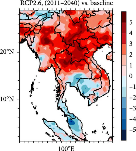
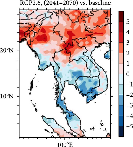
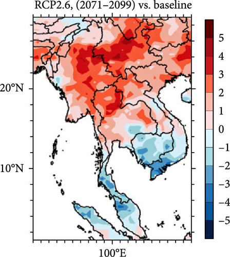
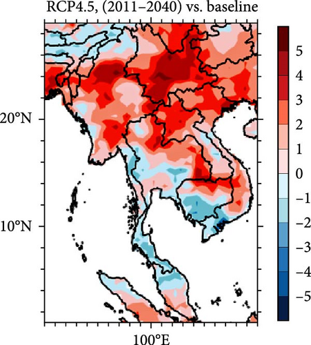
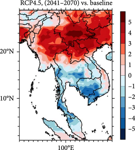
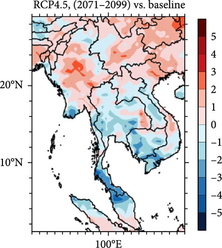
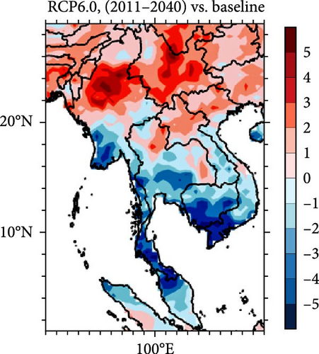
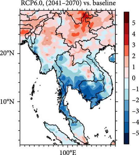
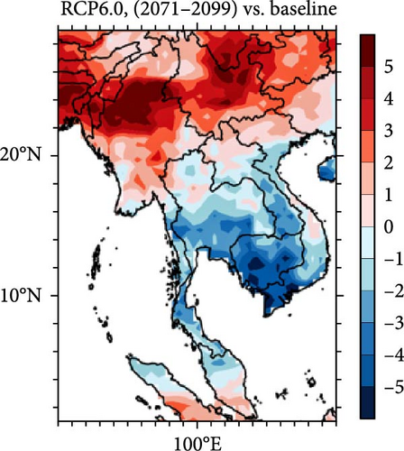
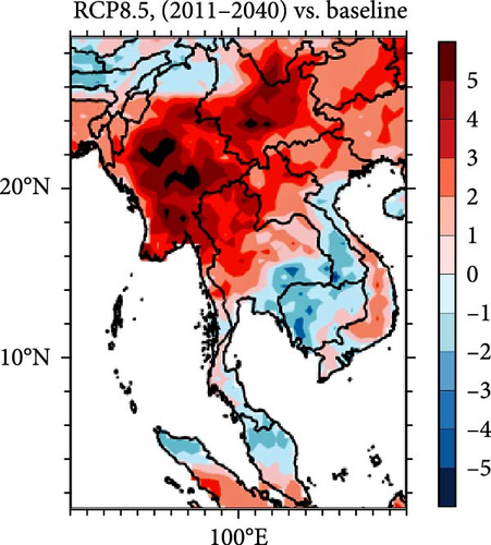
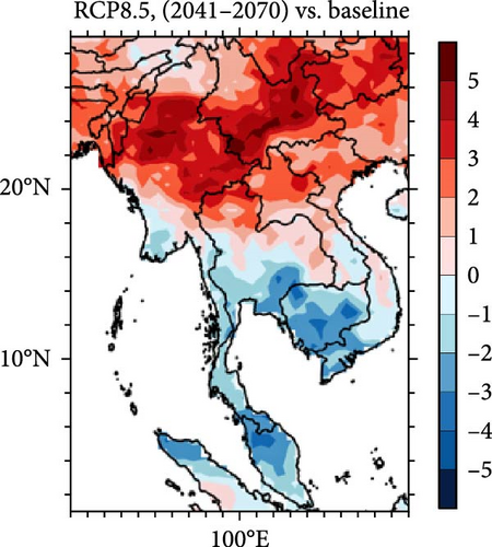
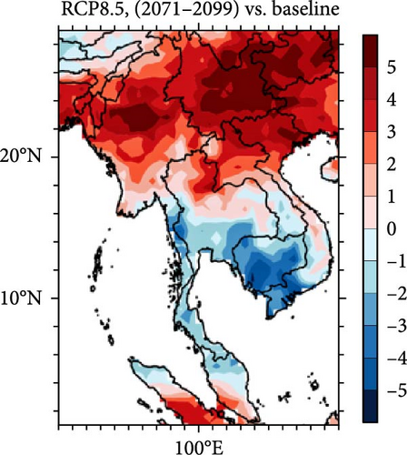
A noteworthy observation pertains to the existence of favorable patterns in CDDs within the northern regions of several countries, such as Myanmar, Laos, Vietnam, and northern Thailand, as indicated by the RCP2.6 scenario. This observation is similar to previous studies conducted by Dai [7] and Huntington et al. [34], which have repeatedly indicated that certain regions are experiencing greater aridity and heightened risk of drought as a result of climate change. These changes can be attributed to rising temperatures and alterations in precipitation patterns. On the other hand, the adverse patterns observed in the CDDs throughout the southern territories, which include Cambodia, Malaysia, and the southern segment of Thailand, within the context of the identical RCP2.6 scenario, give rise to inquiries. Although additional research is required to fully understand the implications of these results, other studies, such as Trenberth et al. [35], have suggested that changes in precipitation patterns resulting from climate change may increase the probability of drought occurrences in these areas. Moreover, the examination of different RCPs scenarios, namely RCP2.6, RCP4.5, RCP6.0, and RCP8.5, demonstrates that the magnitude of change in CDDs is significantly impacted by the emissions scenario selected. The results align with previous investigations conducted by Collins et al. [36] and Knutti et al. [37], highlighting the correlation between distinct RCP scenarios and the diverse magnitudes of global warming and its associated consequences. The RCP8.5 scenario, which projects the strongest radiative forcing, is linked to a notable escalation in CDDs. Furthermore, the fluctuations in CDDs over time, particularly in the RCP2.6 scenario, demonstrate significant alterations during the early years of the century. These findings are consistent with previous research conducted by Dai [7] and Cook et al. [38], which have examined the relationship between climate change-induced aridity and its heightened effects in the short term. The study’s findings highlight the susceptibility of Myanmar to drought caused by climate change, aligning with previous research conducted by Pang et al. [39] that underscores the importance of implementing methods for adaptation to address these changes. Moreover, the presented results are consistent with previous studies by Nastos and Zerefos [18], who investigated the regional and temporal changes of sequential dry and wet weather in Greece. Their findings emphasized the need to understand successive dry day patterns, which can have serious consequences for water supply and agricultural activities.
3.2.2. Maximum Number of CSUs
Distinct changes in the CSUs show that radiation forcing has a major impact on how long summer heat lasts in MSEA from 2011 to 2099 (Figure 5). This indicator counts how many days in the summer the highest temperatures in various RCPs are over 25°C. With the lowest radiative forcing level, RCP2.6, predicts a little rise in CSUs, lengthening summer days by 3 to 6 days per 30 years throughout the region. This little increase under strict climate mitigation measures points to few changes, highlighting the success of strong environmental laws. By comparison, RCP4.5 exhibits more significant changes, especially after 2041, when CSUs lengthen by 12–15 days per 30 years, mostly impacting the northern parts of Myanmar, Laos, Vietnam, and Thailand. This situation suggests that conventional agricultural timings and water resource management may be challenged by much warmer and longer summers brought on by even modest increases in radiative forcing. Regional variation is seen in RCP6.0; CSUs in central Myanmar and Thailand show modest declines in the early century, but notable rises in the northern regions followed in the late century. Reflecting the intermediate level of radiative forcing linked to RCP6.0, this mixed pattern points to a delayed but significant effect of rising greenhouse gas concentrations. The worst-case scenario, RCP8.5, projects significant and steady rises in CSUs over the course of the century. Substantial increases are noted beginning in 2011; northern Myanmar, Laos, Vietnam, and Thailand are expected to have the most substantial changes starting in 2071. With protracted periods of intense heat seriously impacting agricultural practices and ecological balances, this scenario emphasizes the severe effects of unchecked emissions. The significance and spread of the increased summer heat across Southeast Asia are determined in large part by radiative forcing, as this comparative study highlights. For agricultural management to lessen possible disturbances, higher radiative forcing scenarios (RCP4.5 and RCP8.5) indicate increasing heat stress concerns. The lesser effects noted under lower forcing scenarios (RCP2.6 and RCP6.0), on the other hand, highlight the possible advantages of efficient climate change mitigation measures.

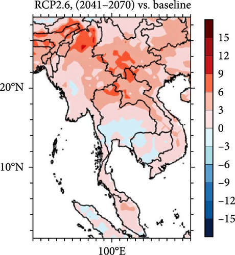
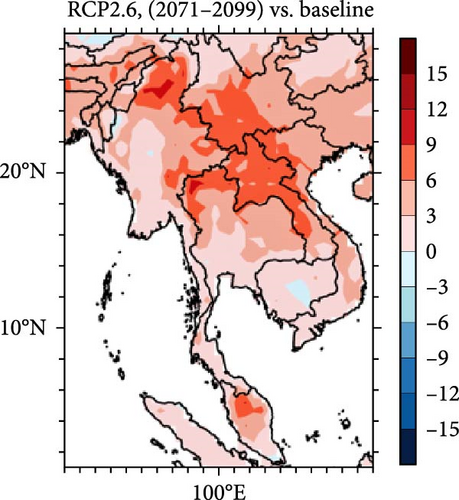
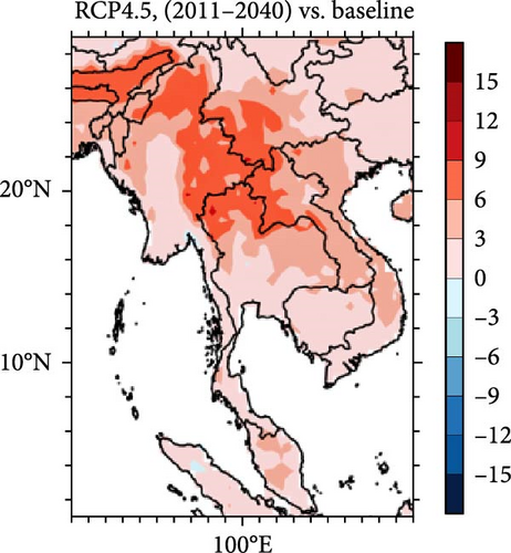
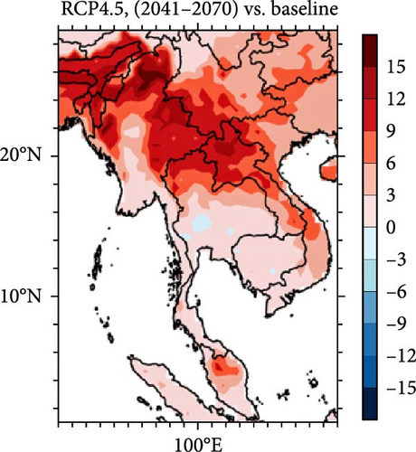
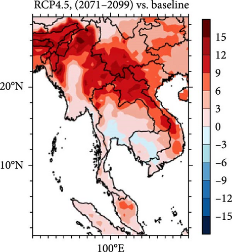
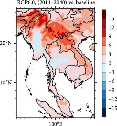
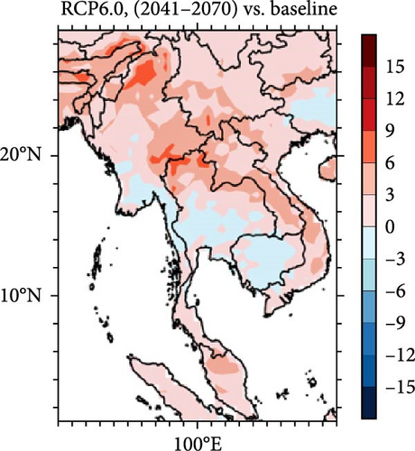
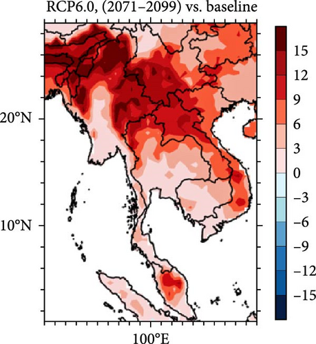
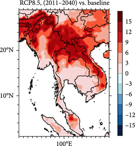
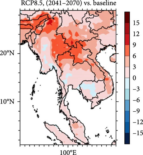
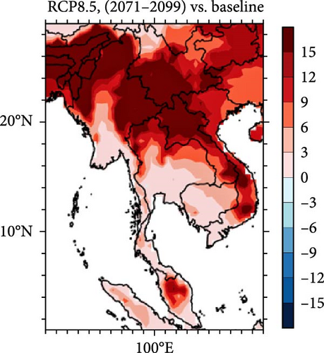
The observed rise in the length of CSUs with temperatures surpassing 25°C, especially in the context of the RCP2.6 scenario, indicates a discernible pattern toward extended and hotter summer periods. This discovery is consistent with prior research that has demonstrated the impact of global warming on the duration and severity of warm episodes [40]. Their study indicates increasing in consecutive dry and hot seasons in MSEA suggests that the region may experience prolonged periods of elevated temperatures and less precipitation. These climatic changes might have significant consequences for multiple sectors, such as agriculture, water resources, and human welfare. The component that is of greater concern is to the amplified scale of change that is anticipated under the RCP4.5 scenario. Notably, there are substantial projected increments in CSUs, particularly in certain regions of Myanmar, Laos, Vietnam, and northern Thailand. This observation is consistent with previous research studies that have indicated an increase in the frequency and length of heat waves because of global warming [41]. The RCP8.5 scenario presents a particularly concerning forecast, indicating a notable rise in CSUs occurrences in northern Myanmar, Laos, Vietnam, and northern Thailand. This observed pattern aligns with the concept that when global temperatures increase, there is a corresponding increase in the frequency of more severe weather events [35]. Moreover, the rise in CSUs may extend growing seasons for certain crops, but it can also intensify heat stress. Crops like rice, which are highly temperature-sensitive during the reproductive phase, may experience reduced grain formation under prolonged heat [42]. On the other hand, heat-loving crops like sugarcane may benefit from longer warm periods [42].
3.2.3. Cold-Spell Duration Index (CSDI)
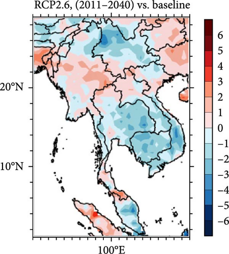
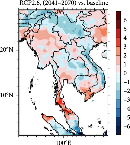
The CDSIs and its variability across several climatic scenarios from 2011 to 2099 clearly show how radiative forcing affects the length of cold spells in MSEA (Figure 6). A little decline in CDSIs occurs under RCP2.6, which has the least radiative forcing, and cold periods are shortened by 1 to 2 days every 30 years, mostly affecting the southern parts of Thailand, Vietnam, Cambodia, and Malaysia. This little drop implies that the frequency of cold periods is somewhat constant under strict climate mitigation efforts, which implies less ecological disturbance. For intermediate levels of radiative forcing, RCP4.5 and RCP6.0, cold period lengths usually decrease by 2 to 3 days every 30 years. The most obvious alterations are found in southern Myanmar, Laos, Vietnam, and central and northern Thailand, where the modest rise in radiative forcing causes discernible but not dramatic shortenings of cold spells. With reductions in CDSIs ranging from 3 to 4 days every 30 years throughout different regions of MSEA, RCP8.5, which reflects the highest degree of radiative forcing, anticipates the largest decline. This dramatic decline emphasizes the serious consequences of high radiative forcing levels, which may drastically change winter temperature patterns and negatively disrupt natural and agricultural ecosystems that depend on cold weather. The degree of radiative forcing and the shortening of cold spells throughout the region are significantly correlated, as this comparison study makes abundantly evident. Higher radiative forcing (RCP8.5) scenarios suggest longer cold spells, which presents difficulties for areas that depend on lower temperatures for the stability of the ecology and agriculture. The little changes noted under the lower forcing scenario (RCP2.6), on the other hand, demonstrate the possible advantages of strong climate action in reducing the effects of global warming.
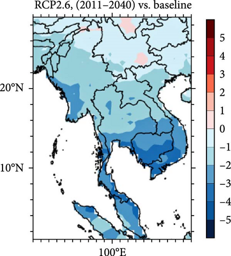
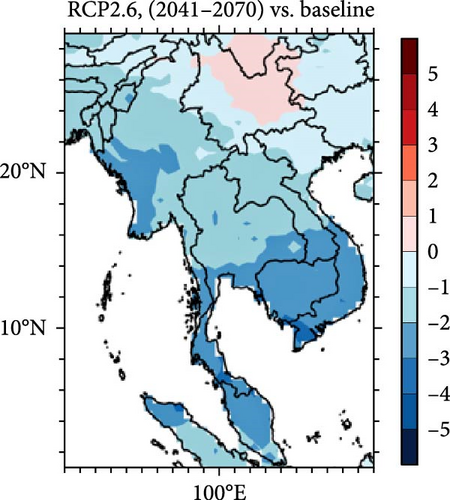
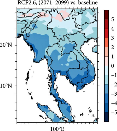
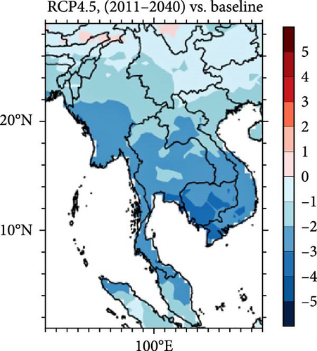
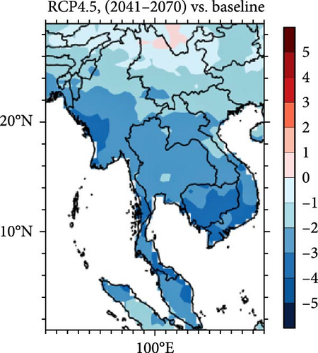
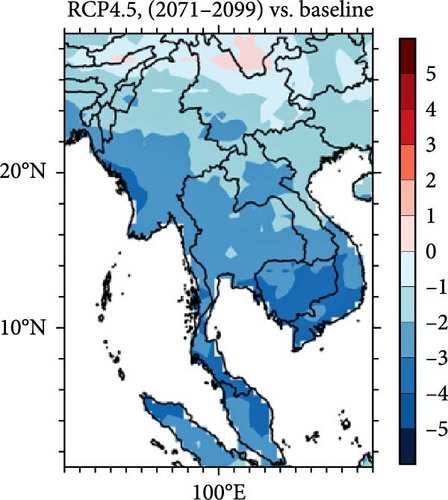
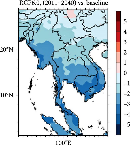


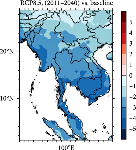
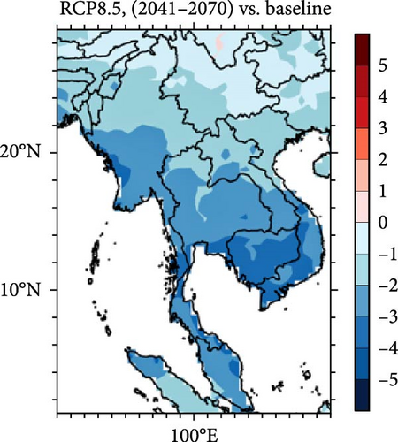
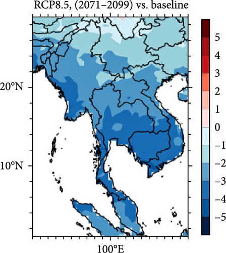
In the RCP2.6 scenario, a discernible decline in CDSIs is observed, with a particular emphasis on the southern regions of Thailand, Vietnam, Cambodia, and Malaysia. Other studies conducted in other places throughout the world have also documented a decline in the occurrence of cold spells, thus underscoring the influence of global warming in modifying temperature patterns [43]. The potential consequences of this prevailing pattern in Southeast Asia may encompass modifications in agricultural methodologies and the transformation of ecosystems that have acclimated to colder climatic conditions. The RCP2.6 scenario expands upon the existing decline in CDSIs, embracing additional geographical areas such as central and northern Thailand, southern Myanmar, Vietnam, and Laos. Cattiaux et al. [44] have also noted a comparable trend of declining occurrences of cold spells in Europe, highlighting the significant impact of climate change on severe temperatures. The prediction based on the RCP8.5 scenario indicates a decline in different Southeast Asian regions, which further supports the anticipation of less severe and shorter durations of cold periods. This statement is in accordance with the prevailing opinion in the field of climate science, which suggests that global temperatures will continue to increase unless substantial measures are made to mitigate this trend [5]. A reduction in the duration of cold spells can influence the cultivation of temperate crops like apples, cherries, and strawberries, which require chilling hours for bud dormancy. The shorter cold periods may also affect the control of pests and diseases that depend on cold winters.
3.2.4. Maximum Number of CWDs
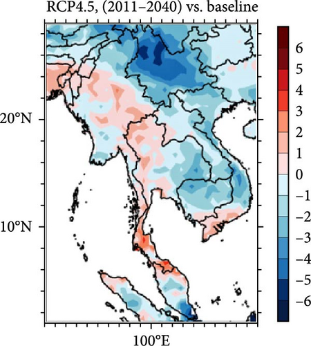
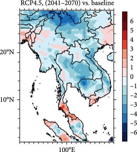
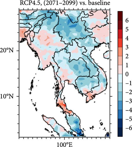
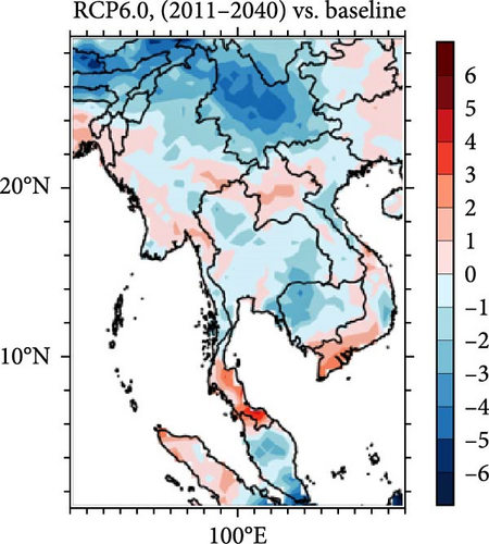
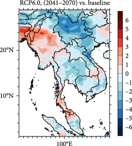
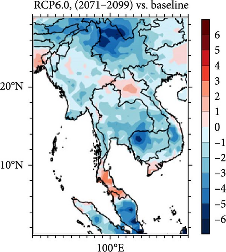
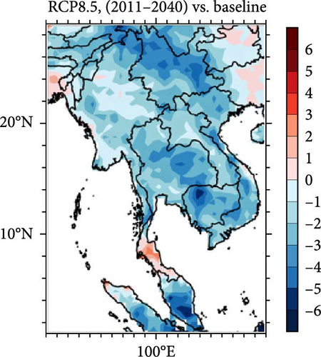
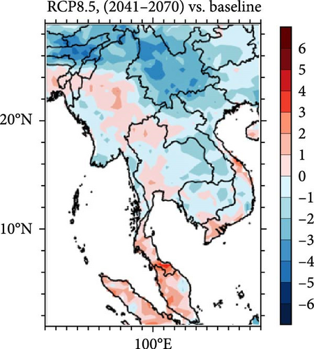
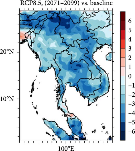
The anticipated decline in CWDs (Figure 7), as indicated by several climate scenarios, is consistent with the predictions of global climate change models that estimate alterations in precipitation patterns [5]. These modifications can potentially have diverse effects, encompassing consequences on agriculture, water resources, and ecosystems. The findings presented in this study align with the global models that anticipate diverse regional reactions to climate change, highlighting the intricate nature of climate effects [36]. With the shifting of precipitation patterns, these regions may encounter difficulties in modifying their plans for water management. According to the RCP4.5 scenario, it is anticipated that the northern region of Thailand will undergo a rise in occurrences of CWDs. The observed decline in the frequency of consecutive rainy days brings attention to the prospective difficulties that may arise in the future for the region, specifically in the domains of water resource management, agriculture, and flood risk mitigation.

3.2.5. WWs
Four climate scenarios—RCP2.6, RCP4.5, RCP6.0, and RCP8.5—are used to illustrate the spatiotemporal variations in WWs from 2011 to 2099 (Figure 8). Significant local differences and trends are shown by this study, which illustrates the direct influence of different levels of radiative forcing on WWs throughout Southeast Asia. With the lowest radiative forcing, RCP2.6, WWs rise steadily but moderately; in Malaysia, for example, they rise by about 5–6 days every 30 years. With little changes in weather patterns, this steady rise points to a steady increase in warmth and moisture that is favorable to longer growing seasons. Specifically in the northern parts of Myanmar, Malaysia, and Southern Vietnam, RCP4.5 predicts more marked increases in WWs, with WWs increasing by 6–7 days per 30 years starting in 2041. This tendency shows that even little increases in radiative forcing can greatly raise temperature and moisture levels, hence affecting agricultural cycles and monsoon patterns. Though at significantly higher intensities, RCP6.0 and RCP8.5 exhibit comparable spatial trends. Particularly, RCP8.5 projects the greatest increases in WWs, up to 10 days per 30 years, in portions of northern Myanmar, Southern Thailand, Malaysia, and the eastern areas comprising Vietnam, Laos, and Cambodia. While in certain places, these large increases may improve agricultural production, and they may also increase the likelihood of flooding and other hydrological effects. By proving a direct link between stronger radiative forcing and higher increments in WWs, the study emphasizes the significant consequences of such situations. This variety emphasizes how complicatedly rising temperatures, more precipitation, and local climatic circumstances interact. Greater radiative forcing scenarios—like RCP6.0 and RCP8.5—are probably going to see bigger increases in WWs, which will provide opportunities as well as problems for regional agricultural and water management. These developments demand for flexible plans to take advantage of any advantages and reduce the risks connected to more frequent rainy days. On the other hand, the less severe effects noted under RCP2.6 highlight the need of strict climate mitigation strategies, which could help stabilize local climates and lower the frequency of extreme weather occurrences.
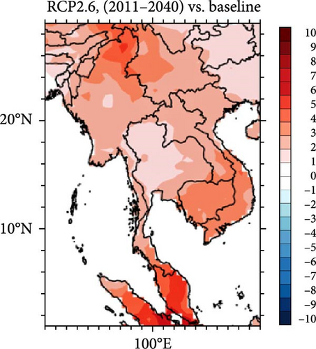
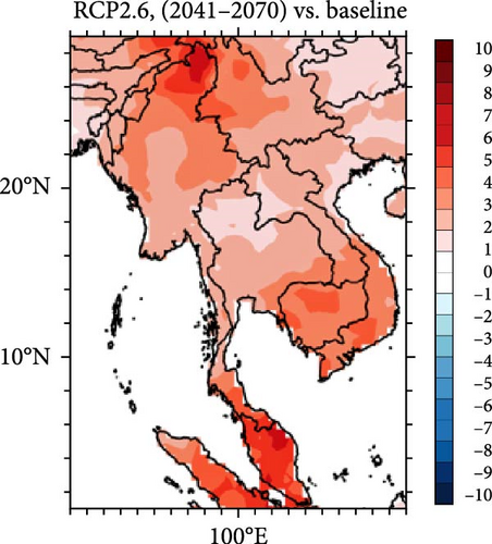
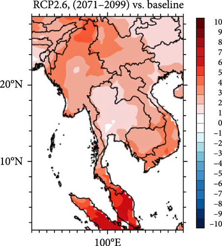
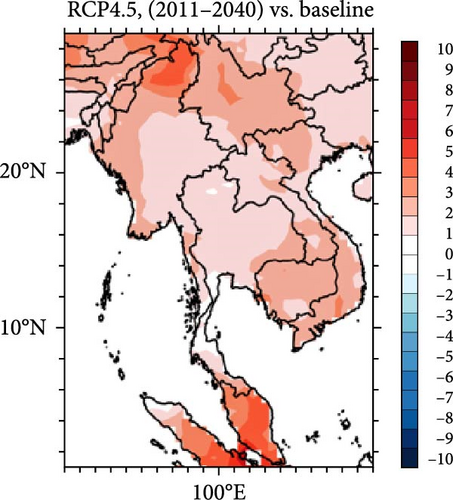
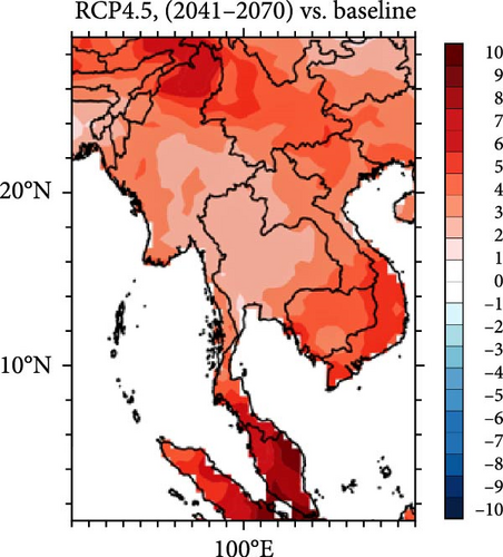
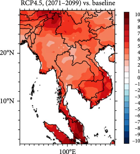
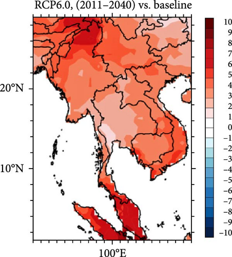
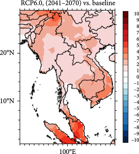
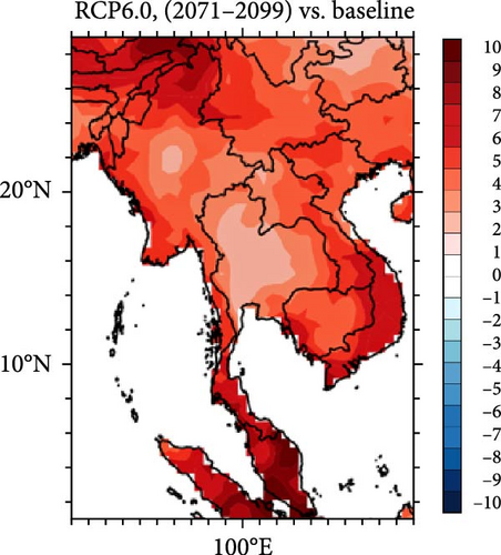

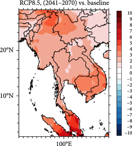
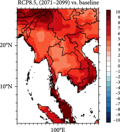
The potential consequences of an increase in WWs include alterations in growing seasons, crop selection, and water management approaches. The RCP2.6 scenario exhibited a notable increase in worldwide warming, with Malaysia experiencing the most substantial jump. The observed significant rise in temperature is consistent with the projections made by global climate models, which anticipate varying regional reactions to climate change. This underscores the importance of implementing adaptation techniques that are tailored to specific localities [36]. The RCP4.5 scenario exhibits a notable upward trajectory in WWs, namely in the northern areas of Myanmar, Malaysia, and southern Vietnam, indicating the possibility of a sustained alteration in precipitation patterns over an extended period. The RCP6.0 and RCP8.5 scenarios exhibit comparable trends of increasing WWs in the northern regions of Myanmar, southern areas of Thailand, Malaysia, and the eastern regions comprising Vietnam, Laos, and Cambodia. Nevertheless, it is worth noting that the increase in magnitude is even more pronounced when considering the RCP8.5 scenario. This observation is consistent with the recognition that different emissions scenarios will result in varied magnitudes of climate change consequences [5]. An increase in WWs can provide favorable conditions for rain-fed crops like soybeans and maize. However, excessive rainfall can also lead to waterlogging and soil erosion, impacting root health and nutrient availability. Rice, which is commonly grown in flooded fields, may be particularly susceptible to water-logged conditions.
In summary, the occurrence of CDDs has been seen to rise in certain locations, particularly in the northern provinces of Myanmar, Laos, Vietnam, and Thailand. This increase in CDDs leads to increased aridity and prolonged periods of dry weather, which can have a substantial impact on the water requirements of crops. This may need an increase in irrigation, which might potentially strain water resources for agricultural purposes, leading to potential impacts on crop output and food security [5]. The small increase in CSUs has the potential to prolong the duration of elevated temperatures experienced throughout the summer season. While there may be advantages for certain crops that have longer growing seasons, there are also issues associated with this, primarily related to the higher rates of evapotranspiration. This may result in the need for more irrigation to adequately fulfill the water requirements of the crops. The reduction in the duration of cold spells, as measured by CDSIs, indicates a shift towards a warmer environment, which has the potential to impact the growth cycles of crops. The rise in the frequency of WWs has the potential to create optimal environmental conditions for specific crops. Nevertheless, the introduction of climate change also brings about a degree of uncertainty in weather patterns, hence emphasizing the criticality of efficient water management practices to mitigate potential problems such as waterlogging and erosion. It is imperative to modify agricultural practices to address these changes, as doing so is crucial for guaranteeing food security and upholding sustainable crop production [10].
3.3. Estimation of CWN for Agriculture
This section has a profound connection to the changes in agroclimatic variables that have been both reported and predicted under different RCPs scenarios. To balance the longer dry spells, for example, the demand for irrigation is expected to rise in tandem with CDDs, especially under higher emission scenarios like RCP8.5. Similar changes in WWs indicate changes in moisture availability, which calls for flexible water management plans to maximize agricultural output and guarantee water sustainability. This part extends the discussion of regional climate effects by converting climatic changes into concrete agricultural water needs. To provide a vital basis for creating responsive agricultural practices that guarantee food security and resource efficiency in the face of climate variability, we examine how these demands can change under various climate futures.
The plots in Figures 9, 10, 11, and 12 illustrate the CWNs in several regions, namely Myanmar, northern Thailand, eastern Thailand, and Cambodia. The data spans numerous time periods, specifically 1981–2010, 2011–2040, 2041–2070, and 2071– 2099. These projections are based on different climate scenarios, namely RCP2.6, RCP4.5, RCP6.0, and RCP8.5. In a broad sense, CWNs exhibit a consistent pattern across various climate situations. The data primarily indicates positive values during the rainy season (May–October) in all regions. However, it was observed that certain months during the dry season, such as March and November, exhibited negative values. In Myanmar, the CWNs exhibit a consistent pattern of positive trends throughout the entire period, particularly from 2010 to 2040, with the highest recorded values occurring in the months of September and November, reaching a peak of 40 mm/month. Initially, the values of CWNs ranged from (−1) to 30 mm/month, but subsequently, they fell within the range of 0–30 mm/month from 2011 to 2040. During the middle and end of the century, the values of CWNs ranged from (−1) to 20 mm/month and from 0 to 50 mm/month, respectively. In the eastern region of Thailand, namely during the baseline period in February, there was a significant negative deviation of 20 mm/month in the values of CWNs. In the eastern region of Thailand, from 2011 to 2099, the values of CWNs exhibited predominantly positive trends within the range of 0–80, as per the RCP6.0 scenario. Conversely, in northern Thailand, a negative trend was observed, particularly during the months of May and June, spanning the period from 2041 to 2070. The magnitude of this negative trend was recorded as (−20) mm/month across all scenarios. In Cambodia, a study conducted during the baseline period identified a concerning pattern of CWNs occurring in specific months, namely March, August, and October. The data reveal a predominantly upward trend during the whole period, except for September and October at the conclusion of the century, which had a decrease of (−30) mm/month. This data indicates the presence of an ample water resource suitable for agricultural purposes. In brief, the water supply for agricultural purposes is generally adequate, except for the dry season from the mid-21st century until the end of the century (2041–2099), during which there may be a potential crisis in water availability for agricultural activities.

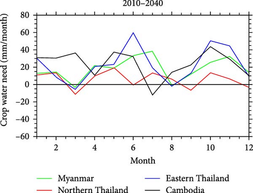
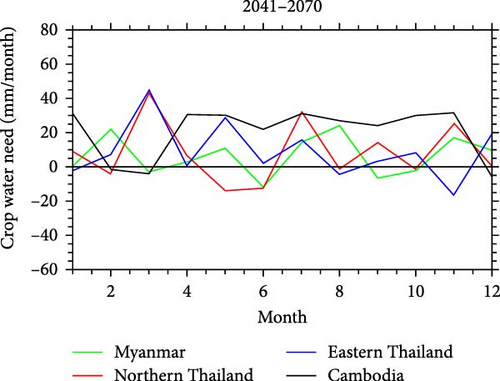
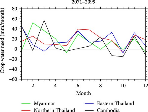

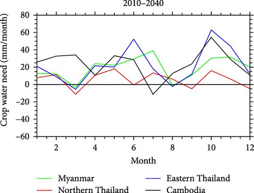
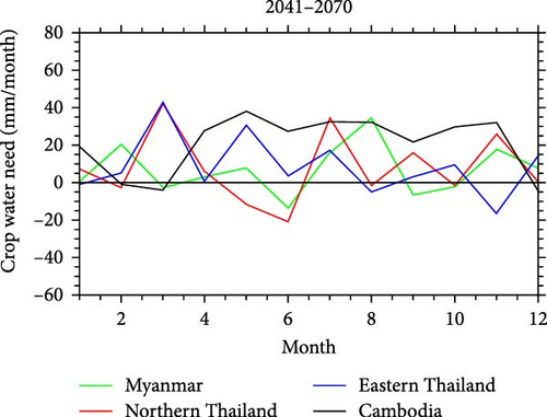
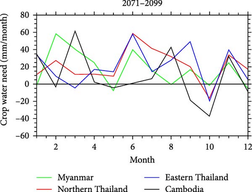

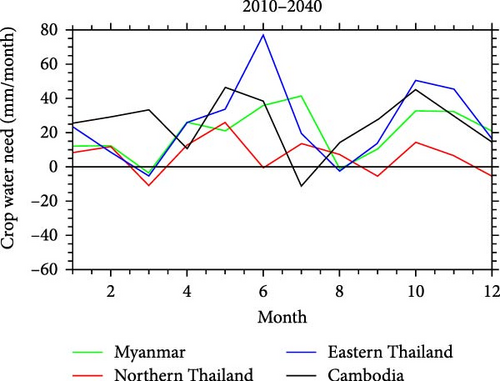
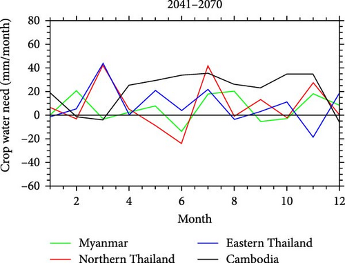
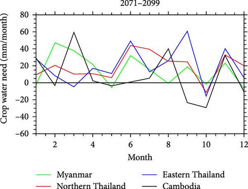
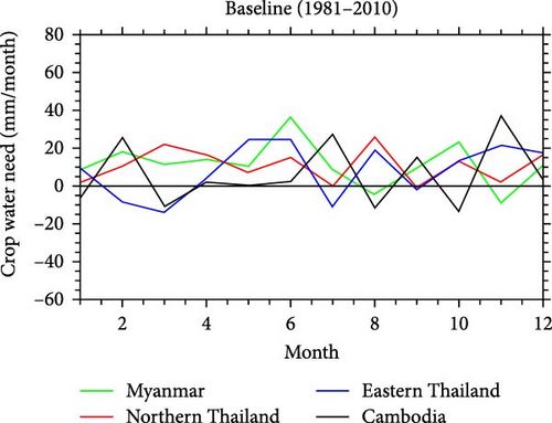
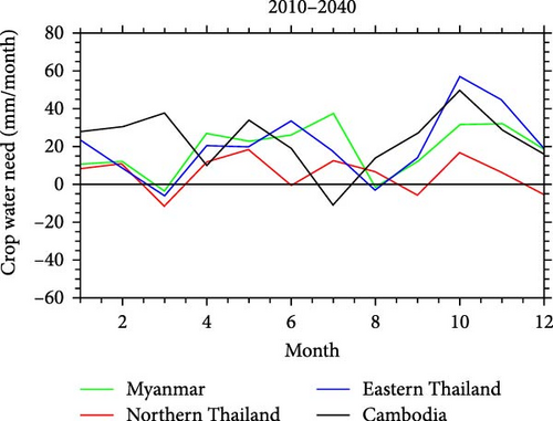
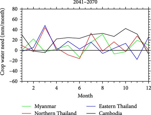
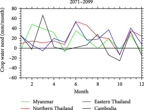
The examination of CWNs in many locations, such as Myanmar, northern Thailand, eastern Thailand, and Cambodia, offers significant insights into the possible water supply and agricultural demands under various climate scenarios. The observed upward trends in CWNs during the rainy season are consistent with the anticipated rise in water requirements for agricultural purposes during this specific timeframe. Nevertheless, the occurrence of negative values in the dry season months, such as March and November, suggests the possibility of water scarcity, which can have substantial ramifications for agricultural output and the stability of food supply [45]. According to Li et al. [46], the demand for water in agriculture may fluctuate over the course of the century, underscoring the importance of implementing adaptive techniques for managing water resources. The seasonal variation in CWNs analysis provides crucial insights into the agricultural water demand dynamics in the regions studied. Positive CWNs throughout the rainy season (May–October) imply an increasing need for water resources to sustain crop growth during this period, which is consistent with Betts et al. [32] findings. In contrast, the appearance of negative CWNs in some dry season months, such as March and November, raises worries about water scarcity during critical crop growth phases. This seasonal variation highlights the importance of implementing adaptive measures such as improved irrigation infrastructure and water conservation methods.
In summary, CWNs are directly influenced by changes in agroclimatic indicators, and understanding this relationship is critical for adapting agricultural techniques in response to changing climatic conditions. The reported increase in the number of CDDs in many Southeast Asian countries, including Myanmar, Laos, Vietnam, and Thailand, indicates an increase in aridity and the extension of dry spells [47]. As a result, there may be a greater need for irrigation and water resources during critical stages of crop development. As agroclimatic indices shift toward drier conditions, it becomes critical to ensure CWNs are met to maintain sustainable crop output. Long-duration of CSUs might potentially have an impact on water requirements. This is because higher temperatures increase evapotranspiration rates, necessitating supplemental irrigation to maintain appropriate soil moisture levels [47]. On the other hand, a decrease in CDSIs suggests a warming pattern, which has the potential to affect crop growing season duration and insect population dynamics. Higher temperatures could increase the growing season, hence producing ideal circumstances for various agricultural crops. Nonetheless, the changing character of the ecosystem may pose new challenges, such as increased pest burdens [9]. The alterations have important implications for CWNs since they may necessitate rescheduling planting and harvesting activities. WWs are becoming more often, which may give favorable environmental conditions for crops. Nonetheless, changing weather patterns create an element of unpredictability, necessitating the installation of rigorous water management measures to handle potential issues such as waterlogging and erosion [10]. The link between agroclimatic indices and CWNs emphasizes the importance of establishing adaptive agricultural systems that adjust for changing climate conditions. Implementing effective water management strategies, such as the use of advanced irrigation systems, the cultivation of drought-resistant crop varieties, and the use of precision agriculture techniques, can help to mitigate the effects of shifting agroclimatic indices on crop water requirements. Implementing these strategies is critical to ensuring food security and promoting sustainable agricultural production in Southeast Asia.
4. Conclusion
This research has delved into a comprehensive examination of agroclimatic indices, including CWDs, CDDs, CSUs, CDSIs, and WWs, and their direct influence on crop water requirements, as represented by CWNs. The GFDL model displayed reasonable accuracy compared to GLDAS, but it tended to underestimate precipitation and exhibited a positive temperature bias. CDDs, CSUs, CDSIs, CWDs, and WWs are among the agroclimatic indicators whose thorough examination this study provides to highlight the relationship between CWN and climate dynamics. We demonstrate that there are significant regional differences in climate effects due to various RCPs. The study particularly points out a rise in CDDs, especially in conditions with stronger radiative forcing, indicating a growing tendency toward aridity and a higher risk of drought in northern Myanmar, Laos, Vietnam, and Thailand. These patterns underscore the pressing need for robust agricultural planning and enhanced water management strategies to mitigate the adverse effects of prolonged dry spells. In a similar vein, the trends seen in CSUs and CWDs point to extended hot spells and changed rainfall patterns that will probably put conventional farming methods and water management plans to the test. Interestingly, we anticipate the CSUs to highlight prolonged periods of heat stress that could negatively impact crop viability and productivity, especially under mid- to high-radiative forcing scenarios. In addition, practical insights are provided by analyzing CWNs in different geographies and climate situations. Though the frequency of negative values during crucial dry season months indicates rising water scarcity that could severely affect agricultural productivity and food security, positive trends in CWNs during the rainy season indicate sufficient water availability for crop development.
Conflicts of Interest
There are no conflicts of interest regarding the publication of this paper.
Acknowledgments
We would like to thank Copernicus Climate Change Service, Climate Data Store (2021): CMIP6 climate projections. Copernicus Climate Change Service (C3S) Climate Data Store (CDS). DOI: 10.24381/cds.dad6e055 for Agroclimatic data based on GFDL data. We also acknowledge the Global Modeling and Assimilation Office (GMAO) and the National Aeronautics and Space Administration (NASA) for GLDAS data. We gratefully acknowledge the European Centre for Medium-Range Weather Forecasts (ECMWF) and the Coupled Model Intercomparison Project Phase 5 (CMIP5) for providing the data used in this study. This research was financially supported by the University of Phayao and Thailand Science Research and Innovation Fund (Fundamental Fund 2024).
Open Research
Data Availability
The agroclimatic data based on GFDL is available at https://cds.climate.copernicus.eu/. The GLDAS data are available at https://giovanni.gsfc.nasa.gov/giovanni/.


