Spatiotemporal Dynamics of a Reaction Diffusive Predator-Prey Model: A Weak Nonlinear Analysis
Abstract
In the realm of ecology, species naturally strive to enhance their own survival odds. This study introduces and investigates a predator-prey model incorporating reaction-diffusion through a system of differential equations. We scrutinize how diffusion impacts the model’s stability. By analysing the stability of the model’s uniform equilibrium state, we identify a condition leading to Turing instability. The study delves into how diffusion influences pattern formation within a predator-prey system. Our findings reveal that various spatiotemporal patterns, such as patches, spots, and even chaos, emerge based on species diffusion rates. We derive the amplitude equation by employing the weak nonlinear multiple scales analysis technique and the Taylor series expansion. A novel sinc interpolation approach is introduced. Numerical simulations elucidate the interplay between diffusion and Turing parameters. In a two-dimensional domain, spatial pattern analysis illustrates population density dynamics resulting in isolated groups, spots, stripes, or labyrinthine patterns. Simulation results underscore the method’s effectiveness. The article concludes by discussing the biological implications of these outcomes.
1. Introduction
Mathematical modeling is an effective tool for describing and comprehending the complex systems’ spatiotemporal dynamics. The behaviours of various species in the natural ecosystem reveal a wealth of dynamical traits. The habits of different species in the natural ecosystem exhibit a wide variety of dynamic characteristics [1]. Many species have threatened extinction in recent decades as a result of inadequate resources, overexploitation, pollution, and predation. Most species extinctions are caused by an imbalance in the environment or an ecological system. External support trends to prevent species extinction including refuge and population limitation to a single place [2–4]. Considering the issue of extinction, many authors [5–10] investigated the dynamical behaviour of the same system. However, because we live in a spatial environment, spatial aspects in predator-prey systems should be considered. As a result, to characterize these systems, reaction-diffusion equations [11] should be used. The interaction between prey and predators receives the most attention in the ecosystem because it is so important and happens all over the world [4, 12]. In the realm of ecology, the dynamics of predator-prey interactions have long been the focus of interest and research. For forecasting and controlling ecosystems as well as deciphering the complex interspecies balance, it is essential to comprehend the spatiotemporal dynamics of these interactions. Mathematical models may be used as a useful tool for analyzing and forecasting the behaviour of predator and prey populations, which is one way to investigate these dynamics [13].
The spatiotemporal dynamics of a response diffusive predator-prey model is an important study area for a number of reasons [14–16]. First of all, it enables us to investigate the intricate interplay of species in a vast ecosystem. We may investigate how the movement and dispersal of predators and prey affect their population dynamics, geographical distribution, and overall stability by introducing diffusion factors. Furthermore, this study issue is extremely important in the light of global environmental changes and habitat fragmentation [17–19]. Landscape changes and the loss of habitat connectivity can have a significant impact on the dynamics of predator-prey interactions. We may acquire insights into the resilience and susceptibility of ecosystems under changing conditions and improve conservation policies aiming at maintaining biodiversity by examining the spatiotemporal dynamics of predator-prey models. Finally, the study of the spatiotemporal dynamics of a response diffusive predator-prey model is an extremely interesting research area. We can acquire a better understanding of how spatial dynamics and mobility impact the stability, coexistence, and persistence of predator and prey populations by including diffusion variables into mathematical models. This study’s findings have implications for biodiversity conservation, ecosystem management, and our general knowledge of complex spatiotemporal systems in nature and beyond [20, 21].
The creation of spatiotemporal patterns is significant in describing the dynamics of interacting populations as part of a larger ecological community [22, 23]. Such populations are scattered heterogeneously over their habitats, resulting in patterns that might be stationary or nonstationary in terms of time. Turing [24] demonstrated that diffusion-driven instability might bring out the spatial patterns in a system of coupled diffusion equations. Segel and Jackson [25] proved that Turing’s theories can also be applied to species diversity. Gierer and Meinhardt [26] also demonstrated a biologically justified formulation of the Turing-type model. Levin and Segel [27] proposed spatial pattern formation as one of the possible causes of planktonic flakiness.
Nevertheless, when compared to two-species food chain models, pattern development for three-species systems has received far less attention. In the study in [28], White and Gilligan give adequate conditions for a diffusive model to induce diffusion-driven instability. Chen and Peng [29] established the existence of nonconstant positive steady conditions to prove the endurance of static patterns for a cross-diffusion model. They also showed that without cross diffusion, the corresponding model fails to deliver any stationary pattern.
The time-dependent spatial patterns can be studied using the amplitude equation. It offers us a diplomatic classification of weak nonlinear studies’ pattern formation. It is feasible to derive the given model’s amplitude equation using multiple-scale analysis.
A wide range of computational approaches has been employed for the nonlinear prey-predator model, including the finite difference method [30], B-spline method [31], finite element method [32], spectral method [33], perturbation method, variational iteration method (VIM) [34], and so on. Researchers, on the other hand, have always sought to identify the most effective numerical method [35]. A sinc function interpolation method for the prey-predator system has been developed.
In this article, our objective is to explore the intricate spatiotemporal dynamics exhibited by models involving three interacting species (specifically, two prey species and their shared predator). Our primary focus lies in analyzing the consequences of the stochastic dispersal of all three species on their respective population distributions. In addition, we aim to delve into fundamental ecological inquiries, such as the phenomenon of extended transience and the influence of habitat size on the resulting patterns. To address these questions, we thoroughly examine a temporal model based on reaction-diffusion principles. These systematic investigations hold values in discerning and contrasting the ensuing dynamics and their underlying causal factors, given that these three models form a sequence of nested systems. The following is a breakdown of the structure of our work. In Section 2, we introduce a temporal model with three species—two prey species and one predator, and discuss the dynamical behaviours briefly as well as provide stability of the model then expand by including spatial components, where we also present a broad range of spatiotemporal dynamics that the model is capable of. The necessary condition of Turing instability as well as bifurcation is identified in Section 3. In Section 4, a sinc interpolation approach has been developed using our model. We obtain the amplitude equation by applying a weak nonlinear analysis close to the parameter threshold value for the patterns in Section 5. In Section 6, we perform numerical simulations to support our analytical results. Then, we show the Turing patterns for some fixed parameter values in Section 7. We discussed and concluded our work in Section 8.
2. Temporal Model and Stability
The parameters used in the model are described in Table 1.
| Parameters | Description |
|---|---|
| a1(t) | Prey 1 population |
| a2(t) | Prey 2 population |
| b(t) | Predator population |
| g1, g2 | Intrinsic growth rate |
| Carrying capacity of preys | |
| σ, φ | Competition rates between two preys |
| ν, η | The rate of predation on preys by predator |
| μ1, μ2 | Conversion efficiencies of preys |
| ϱ | Predator’s natural death rate |
Theorem 1. E0 = (0,0,0) of system (1) is always a saddle point.
Proof. The Jacobian matrix of (1) about E0 = (0,0,0) is as follows:
The eigenvalues of the matrix are Λ1 = g1, Λ2 = g2, and Λ3 = −ρ. Here, Λ1 > 0 and Λ3 < 0. As a result, system (1)’s equilibrium point is a saddle point.
Theorem 2. of system (1) is asymptotically stable if and . Otherwise E1 is a saddle point.
Proof. The Jacobian matrix for E1 is given by the following equation:
The eigenvalues of the matrix are .
Hence, E1 is asymptotically stable when the restrictions and Kμ1ν < ρ hold and unstable when and Kμ1ν > ρ.
Theorem 3. of system (1) is asymptotically stable if and . Otherwise E2 is a saddle point.
Proof. The Jacobian matrix for E2 is given by the following equation:
The eigenvalues of the matrix are .
Here, Λ1 < 0. If , then Λ2 < 0 and if , then Λ3 < 0.
Therefore, E2 is asymptotically stable if the above condition holds, otherwise E2 is a saddle point.
Theorem 4. of system (1) is asymptotically stable if υ1 > 0, υ2 > 0, υ3 > 0, and υ1υ2 − υ3 > 0.
Proof. At E3, the Jacobian matrix is given by the following equation:
The characteristic equation is as follows:
This can be written as follows:
The equilibrium point E3 is stable by the Routh–Hurwitz criterion if υ1 > 0, υ2 > 0, υ3 > 0, and υ1υ2 − υ3 > 0.
Proof. The Jacobian matrix at E∗ of (1) is as follows:
The characteristic equation is as follows:
This can be written as follows:
The stability of (1) in the nonspatial case is described in details above. Then, the Turing instability of system (1) will be investigated by incorporating diffusive terms.
3. Spatiotemporal Model and Bifurcation Analysis
Here, Λ is a bounded domain in R2 with the smooth boundary ∂Λ∗; ∂/∂n represents the outward drawn normal derivative on ∂Λ∗ while n is the outward unit normal vector of ∂Λ∗. The densities of the three species are denoted by a1(x, t), a2(x, t), and b(x, t), respectively, at spatial position x and time t. The positive parameters di (i = 1, 2, 3) denote the diffusion coefficient of the species.
Here, R0 > 0 if σφa1a2r∗ < p∗q∗r∗ + η2a2μ2bp∗ − σφa1a2r∗ + σηa1a2μ1νb + νφa1a2μ2ηb + μ1ν2a1bq∗ and R1 > 0 if .
Hence, if R3 > (R0 + R1 + R2).
is a criterion for Turing bifurcation spatial patterns if all other mentioned conditions have been met.
In the next section, system (2) can be solved by using the sinc interpolation method as follows.
4. Interpolation Method
The sinc method is a very effective numerical technique [36]. It is frequently used in many different areas of numerical analysis, including quadrature, integral and differential equation solution, and interpolation [37]. When singularities or unbounded domains are present, the method may effectively handle them. As the number of bases rises, the method’s error converges exponentially to zero.
To get the numerical solution of (19), we use the numerical scheme NDSolve in Mathematica software for solving various initial conditions.
The Turing patterns near the bifurcative value were described using amplitude equations. For the aforementioned models, the dynamics obtained by varying the bifurcative values were interpreted using weak nonlinear analysis in the following section.
5. Amplitude Equation and Stability Analysis
In this section, to obtain the amplitude equations that make up the various Turing patterns, we will use the multiple-scale analysis method. We can then determine the necessary conditions for the appearance of various Turing patterns by examining the stability of the amplitude equations, allowing us to construct various Turing patterns through numerical simulation.
Let us now consider the ϵ2 case. By Fredholm’s solubility condition, the vector function of the preceding equation must be orthogonal to the operator ’s zero eigenvectors.
We examine the stability properties of the amplitude equations using (57).
Theorem 6. The prerequisite for stationary state stability is and the condition for the unstable is , where .
Proof. Consider the stationary state to be (O), and from (57), the prerequisite for stability is given by ς1 = ς2 = ς3 = 0 for and for it is unstable.
Theorem 7. The prerequisite for stability for stripe patterns is and unstable if where .
Proof. Let us denote the stripe pattern as (M) and it is given by and ς2 = ς3 = 0.
Consider ςj = ςm + θςj and j = (1,2,3).
Substitute ς1 = ςm + θς1, ς2 = θς2, and ς3 = θς3 in (57) and replace the steady state condition. The following are the mathematical relationships:
The characteristic equation for stripe pattern stability is deduced from (58) as follows:
Substituting in (64), we get the following:
We have λ1 = −2Ω∗ and .
If the eigenvalues are negative, the stripe patterns are stable as follows:
Thus, the prerequisite for stability for stripe patterns is and unstable if .
Theorem 8. The hexagonal pattern is stable if and unstable if , where .
Proof. Substituting ς1 = ς2 = ς3 = ςh in (57), we get the following:
On the basis of the real value, the value of discriminant must be positive and it becomes the following:
Substitute ς1 = ςm + θς1 and ς2 = θς2, ς3 = θς3 in (57) and replace the steady state condition. The following are the mathematical relationships:
From (64), the characteristic equation is as follows:
After solving the above cubic equation, the following eigenvalues are obtained:
Let us examine eigenvalues’ stability conditions, say and .
Case 1. :
Substituting from (62) in λ1 defined as , we get the following:
Assume λ2 = λ3 < 0.
On simplification, we get the following equation:
Thus, the hexagonal pattern is stable if .
Case 2. :
Substitute from (62) in λ1 defined as , we get the following:
On comparing (67) and (70), λ1 is positive. Now, calculating λ2 and λ3, we get the following:
Again comparing (68) and (71), we get (71) as positive.
As a result, when , all eigenvalues turn positive, which assures the instability of hexagonal patterns.
Now, the system can be simulated numerically in a 350 × 350 2D square lattice.
6. Numerical Computation
Analytical studies are never completed unless the results are numerically validated. System (2) is simulated by the ODE solver, and the results are displayed with parameter values. Various numerical results are shown to validate the analytical stability analysis presented in the preceding sections. The analyses have been carried out with positive parameter values. As shown in the images below, we use a variety of parameter values to acquire a better understanding of the dynamics of system (2). The numbers specified for the parameters are not based on field data, and they are purely hypothetical parameters meant to depict the system’s dynamic behaviour.
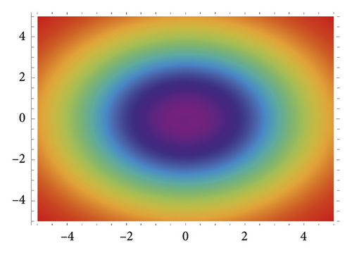
The density plot graph depicts the interplay of prey and predator populations at various geographical regions. Overlapping density plots of both species allow for the identification of locations with more strong predator-prey interactions. Places with high predator density and low prey density may indicate significant predation pressure, whereas places having high prey density and low predator density may indicate prey refuge or favourable breeding grounds.
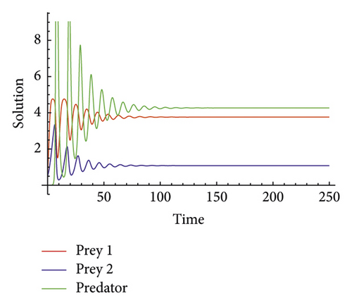
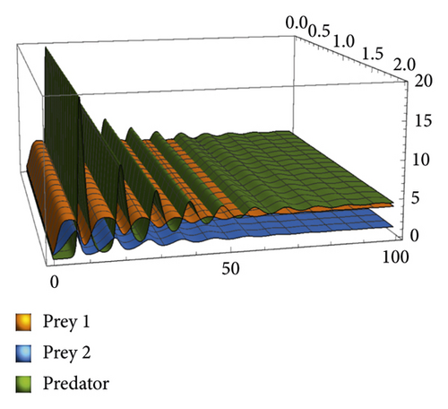
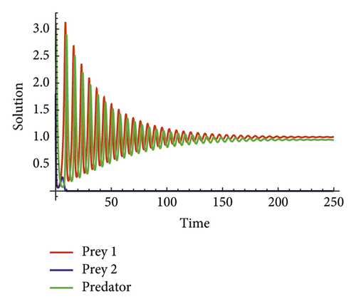
Let us examine model (2) with the following parameter values . From Figures 1 and 2, it is clear that both populations survive for the long term. In addition, Figure 1 demonstrates that the periodic solution emerges for the first prey, second prey, and predator. Consider the same set of parameters as above and slightly change the values of the intrinsic growth rate such that g1 = 1.5 and g2 = 0.5. From Figure 2, it is noticeable that all three species oscillate at a certain time interval then it becomes stable. Figures 1 and 2 are qualitatively equivalent. The outcomes of the remaining instances with instances II and III parameters are qualitatively equivalent. The sole distinction is the duration of the fluctuation period. It appears that being close to steady states is critical, even if the steady state is unstable. Only then can the species cohabit in an oscillating fashion and prevent a large fluctuation (or blooming). It is concluded that prey 1, prey 2, and predator populations coexist simultaneously.
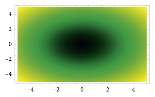
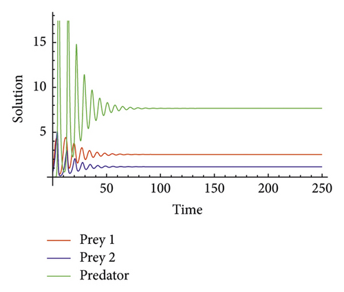
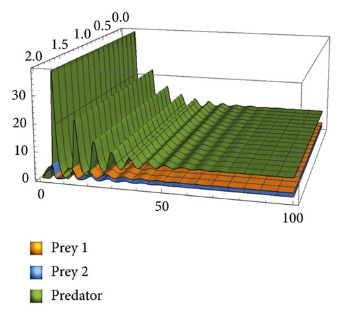
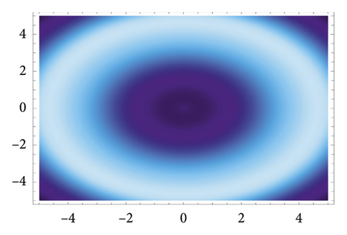
Now, we assume the following parameters . Figure 3, shows that the population persists and are stable.

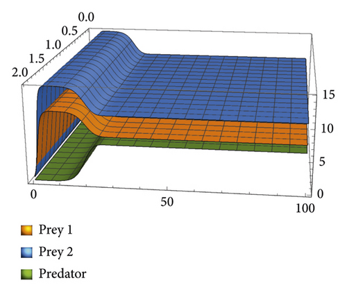
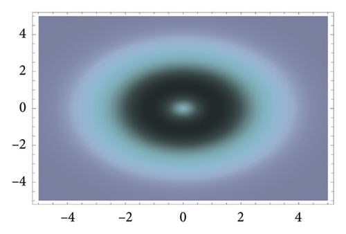
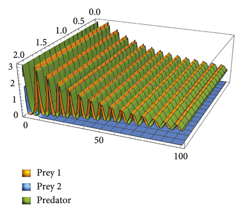
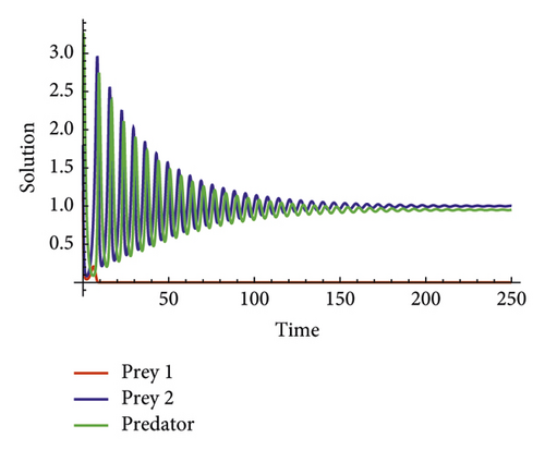
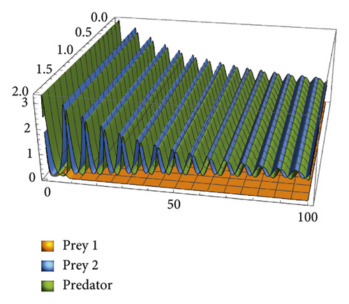
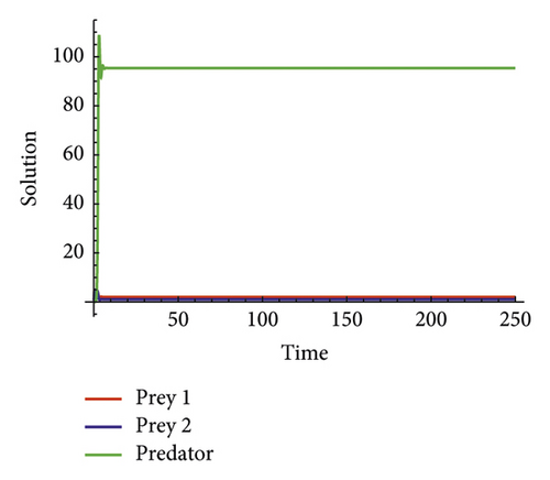
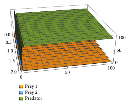
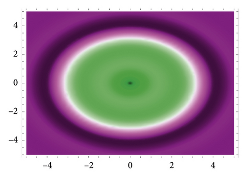
For Figures 4 and 5, let the initial conditions be x0 = 1.2, y0 = 1.8, and z0 = 2.4, and all other constants are 1. From Figure 4, it is noticed that even when is set to a peak value, prey 1 persists at zero level. That is, the prey population vanishes for a large value of , while the other two populations oscillate at time t. Similarly, Figure 5 shows that for the carrying capacity , prey 1 remains at zero level and vanishes. A periodic solution occurs between prey 2 and the predator. The dynamics of the predator species hunting the prey species are also visible in Figure 5(c). The solution consists of multiple layers within the support and generates periodic patterns.
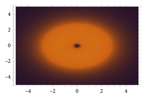
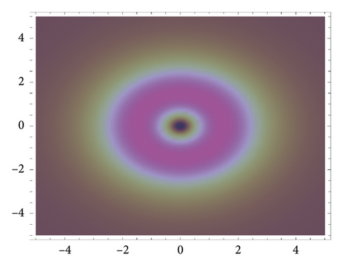
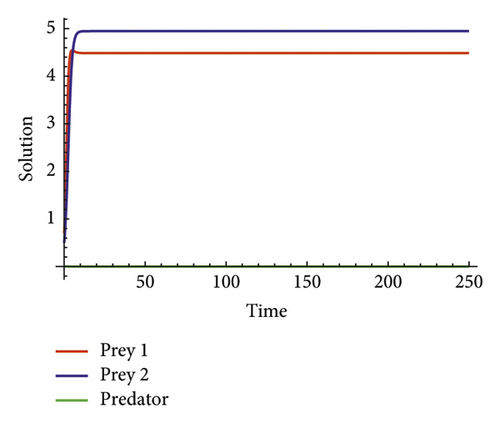
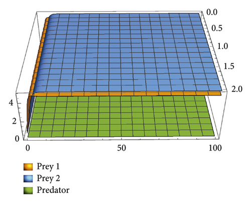
Now, if we decrease the value of the conversion coefficient μ2, it leads to the extinction of the predator, while the prey population remains constant, which is shown in Figure 6. Similarly, from Figure 7, when the growth rate is increased, the prey population disappears while the predator population endures and remains stable. Only circular patterns exist within the solution’s support in Figure 7(c). It is also possible to observe that the predator population is chasing the prey population which leads to the extinction of prey.
7. Pattern Formation
This section examines simulations of system (2) computationally, proving that diffusion creates spatial patterns. Turing patterns can appear in ecological systems as spatially different zones of high and low population densities, resulting in elaborate patterns that resemble stripes, dots, or other complex structures. The appearance of Turing patterns in prey-predator models emphasises the relevance of spatial dynamics and reveals a more complete knowledge of ecological interactions. The emergence of patterns for specific parameter values and diffusion coefficients of (19) is studied, demonstrating how diffusion can cause a stable steady state to become unstable. The simulation proceeds by randomly or predefined distributing predator and prey populations over the geographical region. The system of differential equations is then numerically solved, which advances the populations in time. The diffusion parameters contribute to the expansion of populations at each time step, allowing predators and prey to travel and distribute throughout the domain.
Patterns develop in the population distributions as the experiment proceeds. Depending on the model’s unique characteristics, these patterns might include spatial clusters, waves, or spiral structures. Patterns occur as a result of the intricate interplay between predator-prey interactions, diffusion processes, and the system’s underlying nonlinear dynamics. Contour plots, showing the number of predators and prey at different places, can be used to visualise the simulated patterns. This visualisation gives insights on the population’s geographical organisation and structure throughout time.
We provide here numerical demonstrations to further clarify the prior theoretical results using various sets of parameters. We analyse model (2) by considering the following values, . When the diffusion parameters d1, d2, and d3 are increased from 0.01 to 50, four basic dynamics such as chaos, intermittent chaos, smooth oscillatory state, and stationary behaviour emerge which are shown in Figures 8– Figure 10.
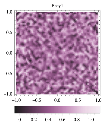
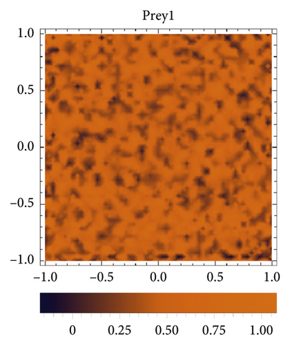
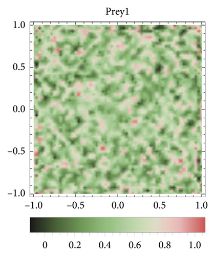
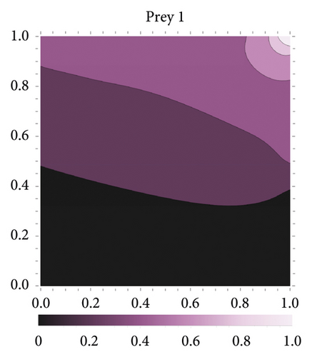
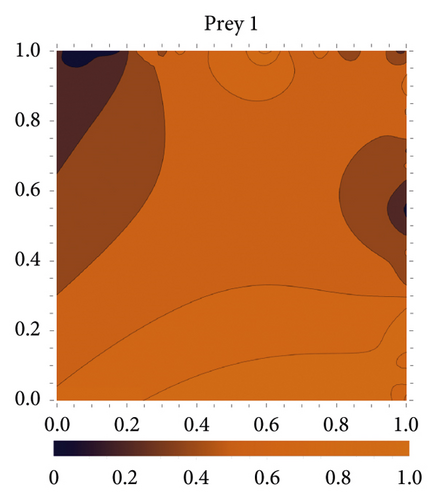
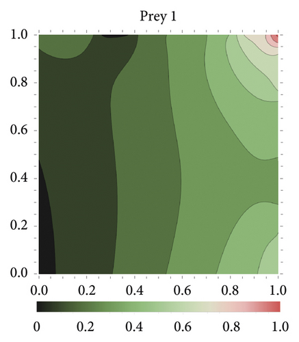
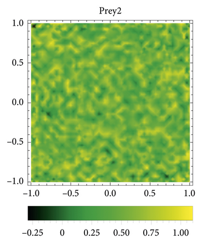
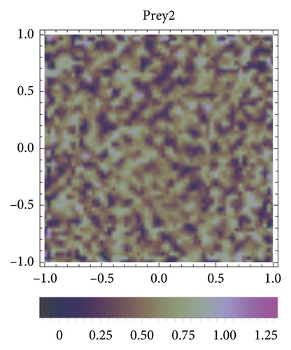
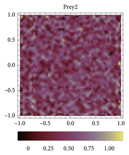
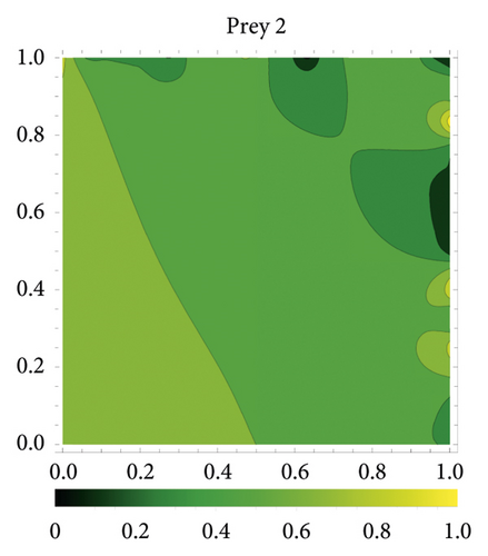
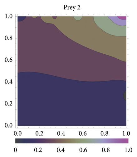
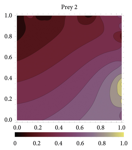
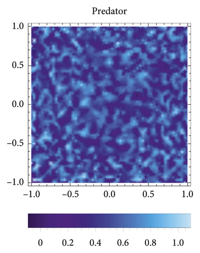
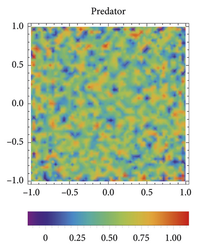
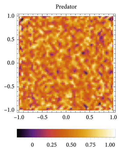
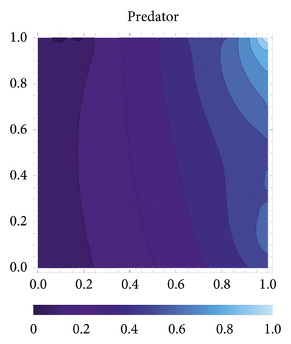
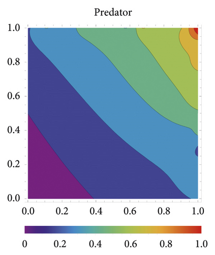
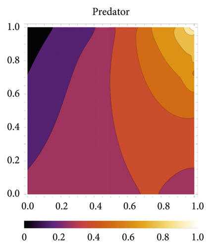
Throughout the prey-predator concept, a pattern is formed when both prey and predator diffuse at different times in three-dimensional space. Figure 11 depicts the coexistence of spot and stripe patterns at intervals of 0, 0.1, 0.2, and 0.8.
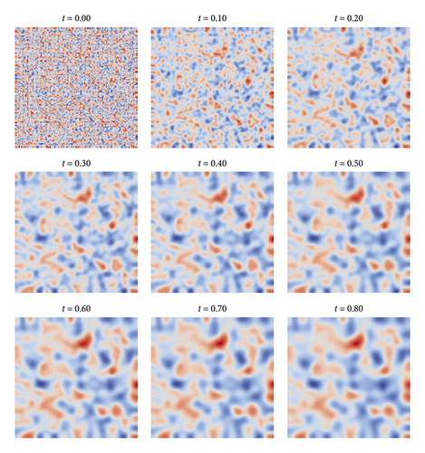
Figure 12 illustrates that predator death rates influence the pattern of spatial distribution. We get a pattern for t = 500 and choose diffusion coefficients d1 = 5 and d2 = 0.2. There are blue and brown spot patterns. In Figure 12(a), blue spots indicate high population density and brown spots indicate low population density, whereas in Figure 12(b), both populations are equal.
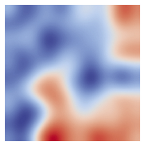

We used Turing patterns in the spatial domain for interpreting system (2). As time passes, the resulting pattern structure will tend to stabilize. The wave number modifies the structure of Turing patterns in homotopy series solutions, which is sensitive to the starting solution. In short, as time goes by in the range of Turing pattern parameters, the system will produce striped patterns, spot patterns, and both striped and spot patterns at the same time.
8. Conclusion
In the present work, we have constructed and explored a predator-prey model characterized by a system of differential equations incorporating reaction and diffusion. Our investigation encompassed an in-depth examination of Turing patterns and spatial pattern formation within the model. We conducted an extensive numerical analysis of the Turing system, investigating how pattern generation is affected by varying parameters. The outcomes included the creation of intricate spatiotemporal patterns, showcasing the spatial complexity attainable in reaction-diffusion systems, including chaotic patterns. We further introduced an innovative sinc function interpolation method applicable to three-species predator-prey systems (PPS) with intricate behaviours. In addition, we have used Taylor’s expansion method to obtain the amplitude equation for the reaction-diffusion system, which accurately described Turing patterns near the bifurcation point. Through simulation results, we successfully demonstrated the effectiveness of this novel approach.
The investigation of Turing patterns in diffusive prey-predator models provides important insights into the spatial organisation and stability of ecological systems. Researchers can get a better grasp of the variables impacting species coexistence, population dynamics, and ecological stability by studying the underlying mechanisms and circumstances that give birth to these patterns. Furthermore, these discoveries have practical applications in sectors such as conservation biology, pest control, and biodiversity protection, where knowing spatial dynamics is critical for making ethical choices. Thus, studying Turing patterns in diffusive prey-predator models is an important area of study in ecological systems. These models improve our knowledge of complicated ecological processes and contribute to the development of sustainable management methods by accounting for spatial dynamics. Further research into the mechanics and consequences of Turing patterns in predator-prey dynamics will surely contribute to a better understanding of the complex interplay between species interactions and geographical variability.
Conflicts of Interest
The authors declare that they have no conflicts of interest.
Acknowledgments
The authors would like to thank the Deanship of Scientific Research, Qassim University for funding publication of this project.
Open Research
Data Availability
No underlying data were collected or produced in this study.


