This paper studies the model-free robust adaptive cruise control problem of a vehicle with unknown nonlinear dynamics and disturbances. First, under backstepping control framework, the position tracking errors with different spacing strategies are used to design a virtual control law, which provides a velocity reference. Then, a novel data-driven sliding surface whose parameters are updated by designing estimation algorithm is developed to handle the unknown uncertainties and disturbances. Finally, the model-free robust backstepping adaptive cruise control (MFRB-ACC) method including PI control, model-free control, and robust control is designed. The novelty of the proposed control technique lies in its strong robustness, which is not based on the precise vehicle model. The designed data-driven sliding surface releases the necessity for the accurate mathematical model of the vehicle and guarantees the inherent robustness of the controller, in particular to uncertainties, modelling error, or external disturbance. Moreover, the designed controller contains three terms such that it has an effective decoupling ability and strong robustness. The effectiveness and superiority of the designed MFRB-ACC method are validated on MATLAB, and the simulation results show that compared to the PID algorithm, the designed MFRB-ACC algorithm can track its preceding vehicle with lower tracking error under different spacing strategies, different operating conditions, and low sampling frequencies. Especially at a sampling frequency of 0.1 s, the error under the PID-ACC increases from 0.2 m at a sampling frequency of 0.01 s to 2 m, and the error under MFRB-ACC has little change compared to the error at a sampling frequency of 0.01 s.

1. Introduction

Adaptive cruise control (ACC), which is an advanced driver assistance system (ADAS), has been attractively studied and equipped in some brands’ high-end vehicles [1]. Unlike the widely used cruise control (CC) which aims to maintain a constant velocity, ACC mainly focuses on tracking predecessor vehicle with a desired distance by adjusting its velocity adaptively [2]. As a consequence, ACC has unique advantages in driver desired response and fuel economy [3]. From the control theory perspective, previous researches about ACC mainly focused on the controller designation with different models, different spacing strategies, different control methods, and their tracking performance, stability, and robustness.

1.1. ACC from Vehicle Model Perspective

At present, ACC mainly adopts one- or two-layer control structure. For the one-layer control structure, a three-order vehicle model is established, where the accelerator and brake pedal of the engine are taken as the inputs, and the position and velocity of the vehicle are taken as the outputs. California PATH Program uses this type of model to develop its controller [4]. For the two-layer control structure, the upper layer determines the desired longitudinal acceleration according to the driving environment, and the lower layer controls the accelerator and brake pedal of the engine such that the vehicle can move with the desired longitudinal acceleration of the upper layer. The lower-layer control can be well achieved using existing control methods. So, the researchers mainly focus on the controller designation of the upper-layer vehicle model. For instance, [5] proposed a model predictive control (MPC) structure to solve the ACC problem with nonlinear vehicle model, where MPC is placed in the upper layer. [6] designed a multiobjective upper-layer controller for ACC under MPC theory, and the designed ACC can solve the problems of fuel economy, tracking capability, and driver desired response. It should be pointed out that the above methods require the accurate vehicle model for controller designation. However, it is impossible to establish the accuracy vehicle model due to uncertainties, disturbances of the mechanism (actuator, sensors, etc.), and interference of the complex external environment (time-varying driving resistance caused by different weather, road, etc.) [7, 8].

In order to avoid the necessity for the accurate vehicle model, neural network and fuzzy logic were used to approximate the nonlinear terms of a vehicle in many kinds of researches. For example, [9] used radial basis function neural networks (RBF NNs) to approximate the unknown driving resistance of a vehicle, and a neural cooperative ACC was designed. [10] adopted a fuzzy model to approximate the preceding vehicle model so that the unknown tracking target was predicted. However, the approximate ability is related to the high-frequency adaptive law and the number of neurons. Besides, PI/PID approaches were applied in various fields without any model knowledge to achieve complex tasks [11]. [12] proposed an intelligent PI feedback/feedforward control scheme to design the ACC system. In the Grand Cooperative Driving Challenge (GCDC), [13] used PID control to design ACC for production vehicles. However, nonlinearities and disturbances of vehicle dynamics are still intractable problems for PID control. So, in practice, PID controller adopts a high-frequency control strategy (usually 0.01 s) to reduce the disturbances of nonlinearities and disturbances. It is clear that both neural ACC and PID ACC require high-frequency sampling and control, which cause great requirements for sensors and actuators. So, it is necessary to design ACC which can release the necessary high-frequency time steps and accurate vehicle model.

1.2. ACC from Spacing Strategy Perspective

Spacing strategy provides reference distance for ACC algorithm; it can be seen as the basic control objective of the ACC. Too small spacing strategy may cause traffic collision. Too large spacing strategy will not only lose the traffic capacity of the road but also can be easily inserted by vehicles in adjacent lanes. So, the spacing strategy has important influence for the tracking performance. There are two main spacing strategies: constant spacing strategy and variable spacing strategy [14]. The constant spacing strategy means that the vehicle moves at a constant distance. This strategy is simple, less computation, and has no interference with the controller designation. But the constant spacing strategy cannot adapt to the complex and changeable driving environment. To solve this problem, variable spacing strategies were widely studied. Representative strategies include time headway-based spacing strategy and human factor distance strategy.

The time headway spacing strategy means that the desired space keeps a linear relationship with the vehicle’s velocity. The greater the velocity, the greater the desired space, and vice versa. Headway is another factor that affects the desired space. If the headway is constant, the spacing strategy is called constant time headway (CTH) [15]. [16] studied the driving performance and traffic flow of the ACC with different values of time headway according to a large number of simulations, and the results shown that different driving environments should adopt different time headway. [17] pointed out that CTH is too conservative in the complex driving environment due to it does not consider the velocity of its preceding vehicle. If the headway is a variable, the spacing strategy is called variable time headway (VTH) [18]. Different from CTH, the time headway of VTH changes with the driving environment [19]. It should be pointed out that the variable space will lead to the variable control objectives and increase the difficulty of controller design. The existing ACC is mainly designed for the specific spacing strategy, which cannot achieve other space requirements. So, it is necessary to design ACC which can achieve the tracking control for different spacing strategies.

1.3. ACC from Control Method Perspective

ACC designation mainly relies on the model-based and approximation-based approaches. Due to the vehicle having complex hydrodynamics with uncertainties and interferences induced by internal equipment and the external environment, accurate vehicle modelling is difficult and even impossible [20]. Thus, the model-based ACC approaches mostly adopt the nominal vehicle model. Specifically, the ACC is designed using nonlinear model predictive control for the nominal vehicle model [21]. Then, to make the ACC system more robust, sensor failure, actuator failure, energy efficiency, and other problems are considered and solved based on the MPC framework [22]. In addition, by linearizing the nonlinear model of the longitudinal vehicle equation of motion, proportional integral (PI), and proportional integral derivative (PID), H_∞, sliding mode-based ACC structures are designed. However, the above results rely on the accurate vehicle model. To improve the control performance for the vehicle with uncertain parameters, the adaptive control approach is used to design the ACC structure [22]. Furthermore, to design the ACC for the vehicle with unknown nonlinear driving resistances and disturbances, approximation-based approaches are used to design ACC by developing fuzzy logic or neural network techniques [23]. For example, [24] used a fuzzy model to approximate the model of the preceding car, and a predictive control scheme was developed by neural network technique for the ACC system. Although many methods have been proposed, there still exist open issues. Specifically, nominal model and system order are required in the above approximation-based and model-based methods.

During the past decades, PI/PID approaches were applied in various fields without any model knowledge to achieve complex tasks. Recently, model-free control was paid more attention due to its advantages in handling nonlinearities with input and output data only [25, 26]. Although the nonlinearities and uncertainties can be handled using model-free control, the robustness of the control system is hardly guaranteed, and it is aimed at being the first-order nonlinear system. Backstepping technique decomposes the high-order system into several first-order systems. The variables of the next level are regarded as virtual inputs, which act on the first-level system. At the same time, the Lyapunov function is established according to the upper-level system to achieve system stability, until the last system realizes control and gets the input [27, 28]. Backstepping technique provides a complete controller design framework for high-order nonlinear systems to study different problems, such as state constraints [29–31], fixed-time stabilization [32], event-triggered control [33], and prescribed performance control [34]. A combination of backstepping technique and model-free control can provide a research line for model-free ACC design. Sliding mode control is usually used to guarantee robustness and has been well applied [35–37]. In [38], a robust fractional-order fast power-reaching guidance scheme was proposed by introducing the fractional-order operator into the sliding surface. In [39], a new robust fixed-time sliding mode control was proposed by using a fixed-time sliding mode observer for the trajectory tracking problem of the flexible joint robot attached to the drone system. To achieve high performance for the flexible joint robot control, [40] developed an adaptive integral sliding mode controller based on a singular perturbation method and two state observers. [41] developed a robust terminal sliding mode control for underactuated flexible joint robot. [42] proposed a cascaded-extended-state-observer-based sliding mode control for underactuated flexible joint robot. [43] proposed a robust fuzzy sliding mode controller for a skid-steered vehicle subjected to friction variations. [44] proposed a model-based chattering-free sliding mode control algorithm to maintain a desired heating value trajectory of the syngas mixture. [45] proposed a mass adaptive control method combined with robust sliding mode control and linear active disturbance rejection control. However, the superiority of traditional sliding mode control methods is based on the prior knowledge of the plant’s accurate model or nominal model, and the plant-model mismatch may determine the magnitude of the discontinuous term in the discrete sliding mode control law.

Leveraging the above analysis, this study is aimed at designing a novel MFRB-ACC for a vehicle with uncertainties and disturbances induced by internal equipment and external environment. The key contributions can be summarized as follows:

(i)
Compared with the existing ACC method using accurate vehicle model, the model-free approach for the actual vehicle dynamics is investigated, where only the input and output data are used to design the controller
(ii)
Compared with the existing ACC method for specific spacing strategy, the designed controller can achieve the tracking control for different spacing strategies
(iii)
Compared with the existing ACC method needing high-frequency sample, the designed controller can achieve the tracking control with low sampling frequency

The rest of this paper is organized as follows: Section 2 presents the problem formulation. Section 3 proposes the ACC method. Illustrative examples are given in Section 4. Section 5 concludes this paper.

2. Problem Formulation

2.1. Vehicle Motion with Disturbances

The dynamics of a vehicle is formulated as

(1)

where

, and

are the nominal position, velocity, and acceleration of the vehicle at time t, respectively. M describes the mass of the vehicle. δ denotes vehicle correction coefficient of rotating mass. F describes the normal driving force of the vehicle. F_f = Mgc_r, F_w = (1/2)c_fA_fρ_av(t)², and F_i = Mgsin(γ) denote the rolling resistance, air resistance, and gradient resistance, respectively. g denotes the gravitational acceleration; c_r is the rolling resistance coefficient; c_f is the air drag coefficient; A_f describes the projected frontal area; ρ_a is the air density; γ is the road slope.

By considering the disturbances, the actual dynamics can be formulated as

(2)

where p(t), v(t), and a(t) are the actual position, velocity, and acceleration of the vehicle at time t, respectively. F describes the actual driving force of the vehicle. w(t) denotes the bounded disturbance to the vehicle.

Using the first-order Taylor expansion, the discrete form of dynamics can be written as

(3)

where T_s denotes the sampling time. p(k), v(k), a(k), F(k), and w(k) describe the sampling values at instant kT_s. ε₁(k) and ε₂(k) are the discretization errors. H(⋅) = (F(k) − F_f(k) − F_w(k) − F_i(k) + w(k))/δ(k)M(k) describes the unknown function induced by uncertainties and the fully unknown parametric dynamics.

The model (3) has the following properties: the mass of vehicle M(t) is time-varying and unknown. The model disturbance w(t) also is time-varying. Thereby, the nonlinear function H(⋅) is time-varying. Thus, the available neural network approaches cannot be simply applied to achieve the vehicle adaptive control.

Property 1. The vehicle (3) satisfies the Lipschitz condition for Δp(k), ΔF(k), and Δw(k), that is, |Δv(k + 1)| ≤ β|Δp(k)ΔF(k)Δw(k)|, where Δv(k + 1) = v(k + 1) − v(k), Δp(k + 1) = p(k + 1) − p(k), ΔF(k + 1) = F(k + 1) − F(k), Δw(k + 1) = w(k + 1) − w(k), and β is a small constant.

2.2. The Adaptive Cruise Objective

The main purpose of the ACC is to maintain the desired distance between the vehicle and its preceding vehicle. Three spacing strategies are usually used to constrain the safe distance and are given by

(i)
Constant space (CS)

(4)

(ii)
Constant time headway (CTH)

(5)

(iii)
Varying time headway (VTH)

(6)

where d(k) denotes the desired safe distance; d^s describes the standstill distance and usually is chosen as 2 − 5m; h is the CTH and usually is chosen as 0.8 − 2s; h(v(k), k) is the varying time headway; a, b, c are the coefficients describing the VTH, and a, b, c are usually chosen as a = 3, b = 0.0019, c = 0.0448.

This study is aimed at tracking the preceding vehicle with the desired distance asymptotically. And the tracking error is defined as follows:

(7)

where p^L(k) denotes the position of the leader and L_p denotes the length of the vehicle.

The control objective is to design a robust control law for the vehicle (3) only using position and velocity data such that

(8)

3. Adaptive Cruise Control Design

In this section, the detailed steps of the designed MFRB-ACC are presented, and the control structure is shown in Figure 1. We proceed as follows:

(i)
The backstepping error is defined, and the virtual control law is designed using backstepping technique for converting distance control to velocity control in Section 3.1
(ii)
The data-driven sliding mode surface is constructed, and the data-driven estimation algorithm is designed to update the parameters of the designed data-driven sliding mode surface in Section 3.2
(iii)
The MFRB-ACC controller, which contains PI control term, feedback control term, and discontinuous control term, is designed to achieve high precision vehicle tracking performance with strong robustness in Section 3.3
(iv)
The stability of the closed-loop vehicle system is analysed using two steps in Section 3.4: (1) the boundedness of the parameters of the designed data-driven sliding mode surface; (2) the reachability of the sliding mode and the convergence of the tracking error

Details are in the caption following the image — **Figure 1**
Open in figure viewer PowerPoint

The MFRB-ACC structure.

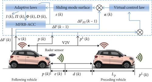
In this procedure, the construction of data-driven sliding-mode surface and the stability analysis are two key points, and we give four theorems to show the main results.

3.1. Backstepping Error

Combing the position tracking error e(k) = p^L(k) − p(k) − d(k) − L_p with (3) yields

(9)

Defining the error z(k) = α(k) − v(k) with α(k) as the virtual control law, then,

(10)

Designing the virtual control law α(k) as

(11)

where k₁ is the designed parameter. Furthermore, we have

(12)

where ξ(k) describes the unknown disturbances, which mainly contain linearization error, the velocity error. Specifically, ξ(k) = ε₁(k) for CS; ξ(k) = ε₁(k) + h(v(k + 1) − v(k)) for CTH; ξ(k) = ε₁(k) + [v(k + 1) − v(k)][c(v(k + 1) + v(k)) + b] for VTH. It is clear that the linearization error exists in all spacing strategies; the velocity error exists in CTH and VTH; and the velocity only exists in VTH. The different spacing strategy leads to the different disturbance, and it is clear that CS < CTH < VTH. The designed ACC must have strong robustness for different spacing strategies.

Leveraging the virtual control law (11), the distance control is transformed to the speed control, and we have

(13)

Thus, the control objective is to stabilize z(k) such that

(14)

It is known that (14) results in the convergence of e(k).

Remark 2. The sampling time and the spacing strategies both have influence for the controller designation. The designed ACC should fully consider these factors.

3.2. Model-Free Vehicle System Description: Data-Driven Sliding Surface

For the vehicle system defined by (3), a sliding mode surface is designed as

(15)

where θ is positive gain; Ω(k) is a time-varying gain defined later; ΔF_PI(k) = K_P(z(k) − z(k − 1)) + K_Iz(k) is PI control law where K_P and K_I are proportional and integral gain, respectively.

Due to the accurate mathematical model of the vehicle, (1) is unavailable for the controller, and the tradition sliding surface (15) cannot be used directly to design the controller. Considering property 1 of the discrete form of vehicle dynamic (3), the data-driven sliding surface is given in the following theorem.

Theorem 3. For the vehicle (3) with unknown dynamics with property 1, there exists pseudopartial-derivative (PPD) Π(k), Φ(k), and Ψ(k), such that when ΔF(k) ≠ 0, the designed sliding mode surface (15) can be transformed as

(16)

where Δα(k + 1) = α(k + 1) − α(k), Δv(k) = v(k) − v(k − 1), |Φ(k)| ≤ κ, |Ψ(k)| ≤ κ, and |Π(k)| ≤ κ.

Proof. Combing (13) and (15), we have

(17)

where

(18)

In some cases, the nonlinear functions G₁(⋅), G₂(⋅), and G₃(⋅) are not differentiable. For example, the mass of sprinkler-car, bus, and some other vehicles change discontinuously.

Case 1: M is smooth, the nonlinear functions G₁(⋅), G₂(⋅), and G₃(⋅) can be differentiated.

In this case, using mean value theorem on (17) yields

(19)

where ∂G^∗/∂p_λ(k), ∂G^∗/∂w_λ(k), and ∂G^∗/∂F_λ(k) describe the gradient values; λ ∈ [0, 1], p_λ(k) = λp(k) + (1 − λ)p(k − 1), w_λ(k) = λw(k) + (1 − λ)w(k − 1), and F_λ(k) = λF(k) + (1 − λ)F(k − 1).

Case 2: M is not smooth, and the nonlinear functions G₁(⋅), G₂(⋅), G₃(⋅) cannot be differentiated.

In this case, define a differentiable function H(⋅) as follows:

(20)

In this way, (19) still can be obtained regardless of the differentiability of H(⋅).

Let Φ(k) = ∂G^∗/∂p_λ(k), Ψ(k) = ∂G^∗/∂w_λ(k), and Π(k) = (∂G^∗/∂F_λ(k)) + (o(k)/ΔF(k)); then, (16) is obtained from (17). Moreover, the defined variables satisfy the inequalities |Φ(k)| ≤ β, |Ψ(k)| ≤ β, and |Π(k)| ≤ β according to Property 1.

The proof of Theorem 3 is completed.

In order to solve the nonsmooth uncertainties and disturbances, time-varying gain Ω(k) is defined as Ω(k) = Π(k), and the data-driven sliding mode surface (16) is simplified as

(21)

where

There are three unknown terms in (21), Φ(k), Π(k), and . These terms affect the cruising effectiveness of the vehicle. Thus, the following data-based estimation algorithm is given.

Lemma 4 (see [26].)For the simplified data-driven sliding mode surface (21) of vehicle (1), the unknown terms Φ(k), Π(k), and could be updated by the following data-driven adaptive laws

(22)

(23)

(24)

(25)

(26)

where

;

, and

are the estimated value of Π(k), Φ(k), and

, respectively.

and

denote the step-size constant.

and

are positive constants.

describes the estimated value of s(k), where

3.3. Robust Controller

The main purpose of the designed controller is to drive the sliding mode surface (15) to the origin, which means

(27)

The model-free robust control laws are designed as follows:

(28)

In detail, the PI control term is given as

(29)

The feedback control term is given as

(30)

The discontinuous control term is given as

(31)

where ρ is a gain constant.

Remark 5. The designed controller contains three terms: PI control, feedback control, and discontinuous control. PI control term ΔF_PI(k) is designed to stabilize the vehicle dynamic (3); feedback control term ΔF_FEE(k) is designed to compensate the unmeasurable, measurable, and unmodelled disturbances; the discontinuous term ΔF_DIS(k) is designed to guarantee the robustness. Thus, the designed hybrid controller has effective decoupling ability and strong robustness.

3.4. Stability Analysis

The stability of the closed-loop system of the vehicle (3) via MFRB-ACC contains two steps. (1) The boundedness of , , and ; (2) the reachability of the sliding mode and the convergence of the tracking error.

Theorem 6. Let the sliding-mode surface be

(32)

with

, and

update by (22)–(26).

, and

are bounded.

Proof. The mathematical induction is used to prove Theorem 6.

Step 1: it is reasonable that the initial conditions satisfy Theorem 6.

Step 2: suppose Theorem 6 holds at instant k − 1, which means , , , and are bounded and for j ∈ 1, 2, ⋯, k − 1, where and .

For the instant k, we have

(1)
For |Π(k)| ≤ φ₁, is bounded according to (24).
(2)
For |Π(k)| > φ₁, by subtracting Π(k) on the both sides of (22), it yields

(33)

where

. According to the definition of Π(k) in Theorem 3, we have |ΔΠ(k)| ≤ 2β.

Leveraging the work of [26], we have

(34)

where

is a constant. In addition, we have

according to the work of [26]. And there exists

and

according to Step 2, where

and

are constants.

Then, we have

(35)

where

Thus, the boundedness of is proved. Using the similar method, the boundedness of can be proved.

In order to analyse the boundedness of , (21) is written as

(36)

where

Defining and and combining (26) and (36), it yields

(37)

Since and are bounded, it can derive that and are bounded according to (36). Thus, there exists a constant such that , where . And it can further yield

(38)

where

. By selecting

and θ,

can be located in (0, 1). The boundedness of

is guaranteed. The boundedness of

is guaranteed due to

. Thus,

is bounded.

Finally, it can be derived that , , and are bounded using the above discussion and mathematical induction.

The proof of Theorem 6 is completed.

In order to proof the convergence of tracking error, (36) is written as

(39)

where

Proposition 7. Define . The term is bounded with the help of Theorem 6, i.e.,

(40)

where

is a positive constant.

Theorem 8. Considering the vehicle (3) under Proposition 7, control law (28), adaptive laws (22)–(26), and virtual control law (11). If ρ is chosen as

(41)

and K_P, K_I, σ, and θ are chosen as

(42)

the asymptotic tracking of a desired trajectory can be achieved using the designed MFRB-ACC, which means that the vehicle can track its preceding vehicle with the desired distance.

Proof. Defining the following Lyapunov candidate function as follows:

(43)

Substituting (28) into (39) yields

(44)

Combining with ((29)–(31) gives

(45)

Similarly, we can derive

(46)

Combining (45) and (46), we have

(47)

Then, it can derive

(48)

For any , it can derive V(k + 1) < 0. Thus, the quasisliding mode is obtained, and s(k + 1) satisfies s(k + 1)⟶0. Furthermore, by combining (15), we have

(49)

where

and

Defining , the solution of (49) can be obtained as follows.

(50)

Since K_P, K_I, σ, and θ are chosen as (2K_P + K_I)(−β + (σ/θ)) < 2, so it can derive

(51)

which further indicates

and

. Consequently,

can be guaranteed. In this condition, the asymptotic tracking of a desired trajectory could be achieved, which means s(k + 1)⟶0. If s(k + 1)⟶0, z(k + 1)⟶0, and e(k + 1)⟶0, which means the vehicle can track its preceding vehicle with the desired distance.

The proof of Theorem 8 is completed.

4. Simulation Studies

In this section, the MATLAB simulations, running on Windows 10 platform with Intel Core i7-11700, 16 G memory, are shown to demonstrate the effectiveness of the designed MFRB-ACC considering three factors: spacing strategies (CTH and VTH), sampling time (T_s = 0.1 and T_s = 0.01), and vehicle moving conditions (cut-out and cut-in). In addition, to illustrate the advantages of the designed MFRB-ACC, the PID-ACC is also used in the examples.

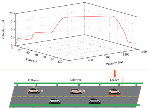
The time-velocity-position profile of the lead vehicle is shown in Figure 2. The parameters of the vehicle are given as follows: M = 3250 + 5000^∗sin(0.01t)kg, L_p = 5m, g = 9.8m/s², A_f = 2.2m², c_r = 0.018 + 0.002^∗sin(t), c_f = 0.35 + 0.005^∗sin(t), ρ_a = 1.2258, γ = 30, and δ = 1. These parameters can only be used to update the vehicle states and cannot be used in the controller.

4.1. Validation of Control Performance for the Spacing Strategy

In order to illustrate the advantages of the proposed controller for the different spacing strategies, the CTH and VTH are set as control objectives for the designed MFRB-ACC and PID-ACC.

4.1.1. Control Performance for CTH

In this example, the spacing strategy is CTH, and the sampling time is T_s = 0.01. The desired distance parameters are set as follows: d^s = 2 and h = 0.8. The designed MFRB-ACC scheme and the traditional PID-ACC method are used to perform the comparison analysis. The initial conditions of vehicle and system states are chosen as follows: p(1) = 0, v(1) = 0, p^L(1) = 2, , , , F(1) = 3, and α(1) = −0.455. The control parameters of MFRB-ACC are chosen as follows: k₁ = 0.1, θ = 0.9, σ = 1, K_P = 2, K_I = 0.1, , , , , ρ = 0.05, and . The control parameters of PID-ACC are chosen as follows: K_P = 50, K_I = 100, and K_D = 50.

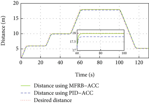
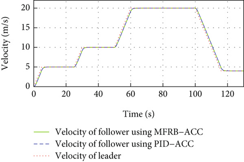
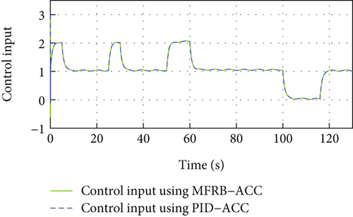
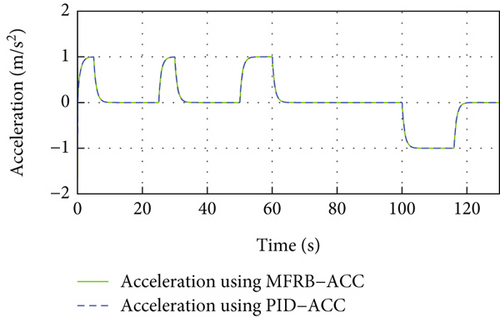
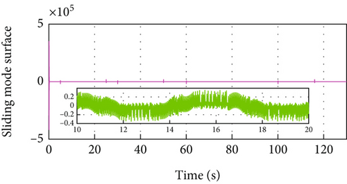
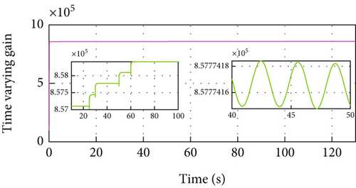
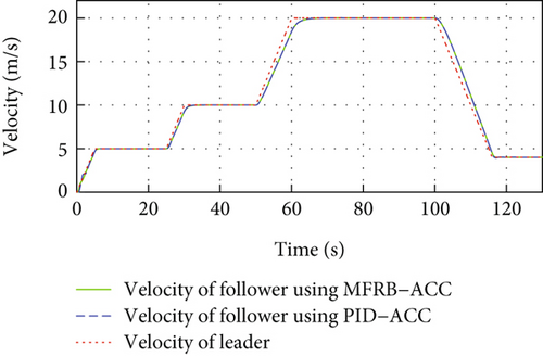
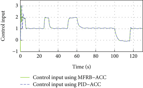
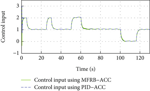
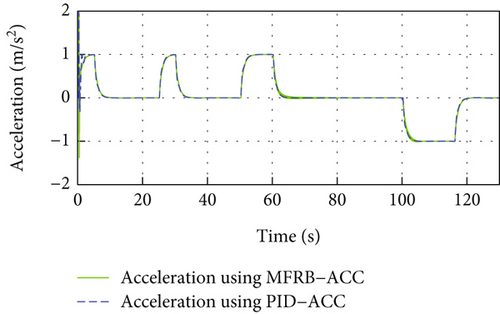
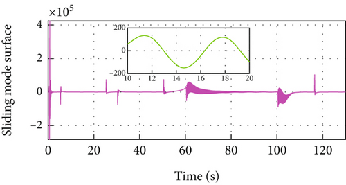
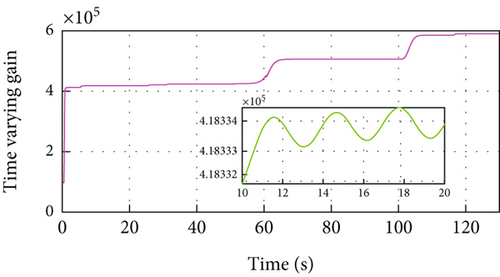
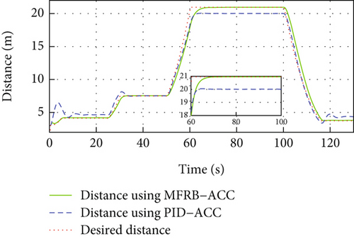
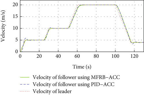
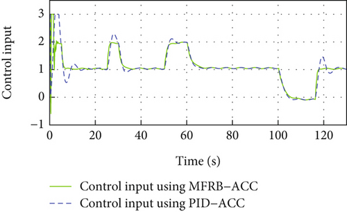
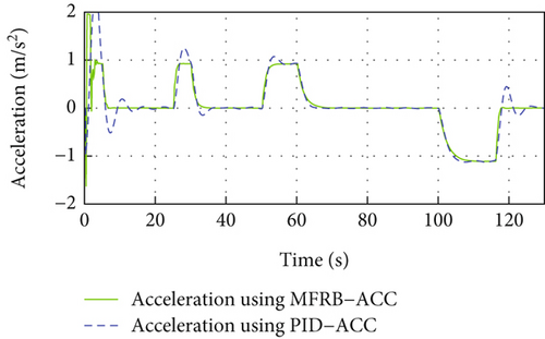
Figure 3 gives the distance, velocity, control input, and acceleration of the controlled vehicle, respectively. The vehicle can security track its preceding vehicle with the desired distance, even if the distance is varying with its velocity. Specifically, the MFRB-ACC exhibits better cruising performance than PID-ACC in terms of tracking precision during 60 s-100 s. In Figure 3(b), when the leader vehicle moves with constant velocity, the follower can track it asymptotically. When the reference trajectory changes, the controller provides corresponding force to accelerate the vehicle; moreover, the control input has no saturation in Figures 3(c) and 3(d). Figures 3(e) and 3(f) show the sliding mode surface and time-varying gain. All of these show that the designed MFRB-ACC can security track its preceding vehicle with good tracking performance and good ride comfort.

4.1.2. Control Performance for VTH

In this example, the spacing strategy is VTH, and the sampling time is T_s = 0.01. The desired distance parameters are set as follows: a = 3, b = 0.0019, and c = 0.0488. The initial conditions of vehicle and system states are chosen as the above example. The control parameters of MFRB-ACC are chosen as follows: k₁ = 0.1, θ = 0.9, σ = 1, K_P = 1, K_I = 0.2, , , , , ρ = 0.005, and . The control parameters of PID-ACC are chosen as follows: K_P = 5, K_I = 10, and K_D = 5.

In Figure 4, same as Figure 3, the developed MFRB-ACC exhibits better cruising performance than PID-ACC in terms of tracking precision during 60 s-100 s. Specifically, the position tracking error using PID-ACC scheme is larger than using MFRB-ACC. The main reason is the influence of unknown disturbances, unknown driving resistances, discretization errors, and backstepping errors. The MFRB-ACC scheme can achieve the full-velocity cruising with the desired distance. The main reason is that the designed decoupled PI-type sliding surface can deal with the disturbances and couplings, and the designed MFRB-ACC can compensate for the unknown nonlinearities. The simulation results demonstrate the decoupling ability and strong robustness of the developed MFRB-ACC scheme. Figure 4(b) shows that the velocity trajectory can track the leader. The control input is smooth, and there is no saturation in Figures 4(c) and 4(d). Figures 4(e) and 4(f) show the sliding mode surface and time-varying gain.

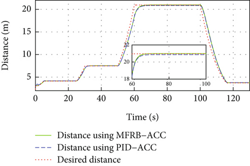
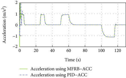
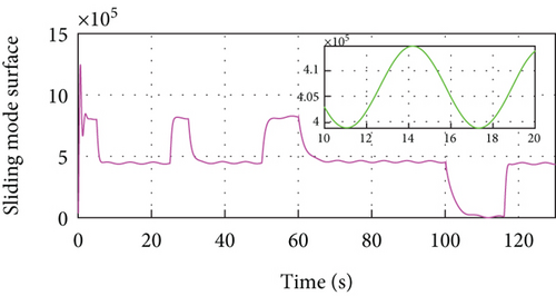
To evaluate the advantages of the proposed MFRB-ACC, Table 1 shows the position tracking error when using MFRB-ACC and PID-ACC, respectively. It is clear that the proposed MFRB-ACC has better control accuracy than PID-ACC.

Table 1. Tracking error when T_s = 0.01.

Sample time		20 s	40 s	80 s
CTH	MFRB-ACC	0.005 m	0.010 m	0.018 m
CTH	PID-ACC	0.050 m	0.100 m	0.200 m

VTH	MFRB-ACC	0.045 m	0.040 m	0.030 m
VTH	PID-ACC	0.055 m	0.050 m	0.100 m

4.2. Validation of Control Performance for the Sampling Time

4.2.1. Control Performance for CTH

In this example, the spacing strategy is CTH, and the sampling time is selected as T_s = 0.1. The desired distance parameters, initial conditions of the vehicle, and system states are set as Example 1. The control parameters of MFRB-ACC are chosen as follows: k₁ = 0.05, θ = 0.8, σ = 1, K_P = 2, K_I = 0.1, , , , , ρ = 0.005, and . The control parameters of PID-ACC are chosen as follows: K_P = 5, K_I = 5, and K_D = 5.

Figure 5 gives the distance, velocity, control input, and acceleration of the controlled vehicle. The PID-ACC cannot guarantee the desired distance. Especially, if the velocity is larger, the tracking error is larger when using PID-ACC. Figure 5(b) gives the velocity trajectory of the vehicle and it can track the leader. The control input is smooth with a small jerk, and there is no saturation in Figures 5(c) and 5(d). Figures 5(e) and 5(f) show the sliding mode surface and time-varying gain.

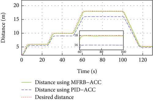
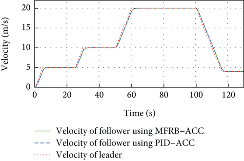
In Figure 5(a) and Figure 3(a), PID-ACC causes errors to increase as sampling time increases, and the developed MFRB-ACC scheme shows better robustness. On the other hand, the relatively small sample time would cost large lots of computing resources. Thus, the sample time in practice should make a compromise between tracking accuracy and cost.

4.2.2. Control Performance for VTH

In this example, the spacing strategy is VTH, and the sampling time is selected as T_s = 0.1. The desired distance parameters, initial conditions of the vehicle, and system states are set as Example 2. The control parameters of MFRB-ACC are chosen as follows: k₁ = 0.05, θ = 0.6, σ = 1, K_P = 0.05, K_I = 1, , , , , ρ = 0.05, and . The control parameters of PID-ACC are chosen as follows: K_P = 2, K_I = 1, and K_D = 10.

In Figure 6(a), the PID-ACC cannot guarantee the desired distance. Same as Figure 5(a), the vehicle cannot track its preceding vehicle with the desired distance, and the tracking error is related with its velocity. Different velocity leads to different position tracking error. The developed MFRB-ACC can security track its preceding vehicle with the desired distance, even if the distance varies with its velocity. It illustrates that the developed MFRB-ACC exhibits the better cruising performance than PID-ACC in terms of tracking precision. Figure 6(b) gives the velocity trajectory of the vehicle. The control input is smooth with a small jerk, and there is no saturation in Figures 6(c) and 6(d). Figures 6(e) and 6(f) show the sliding mode surface and time-varying gain.

To evaluate the advantages of the proposed MFRB-ACC in low-frequency sample, Table 2 shows the tracking error of vehicle when T_s = 0.1. The results show that the proposed MFRB-ACC has better control accuracy than PID-ACC.

Table 2. Tracking error when T_s = 0.1.

Sample time		20 s	40 s	80 s
CTH	MFRB-ACC	0.020 m	0.050 m	0.090 m
CTH	PID-ACC	0.500 m	1.000 m	2.000 m

VTH	MFRB-ACC	0.075 m	0.050 m	0.004 m
VTH	PID-ACC	0.525 m	0.050 m	0.900 m

4.3. Validation of Control Performance for Typical Condition

Above simulations verify the advantages of MFRB-ACC for the unknown vehicle nonlinear running resistances, spacing strategies disturbances, and sampling time errors. This section will test the control performance of MFRB-ACC in different work conditions, such as cut-in and cut-out.

4.3.1. Cut-In Condition

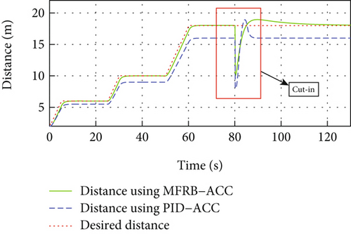
As is shown in Figure 7(a), in this condition, a vehicle cuts between the follower vehicle and the leader vehicle, and the cut-in vehicle will be the new leader vehicle. As a result, the distance between the follower vehicle and the new leader vehicle is smaller than the desired distance. If the MFRB-ACC can make the two vehicles guarantee the desired distance, the robustness of MFRB-ACC can be demonstrated. In this condition, based on the example in Section 4.2.1, when the vehicle runs to 80 s, a vehicle cuts between the follower vehicle and the leader vehicle, and the distance between the follower vehicle and the new leader vehicle decreased by 8 m.

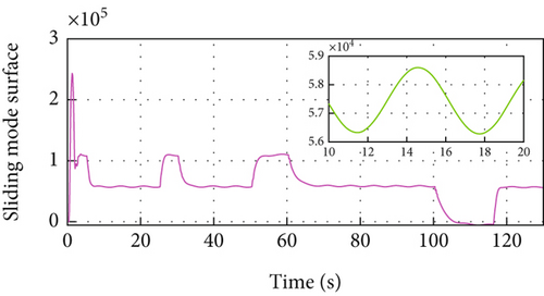
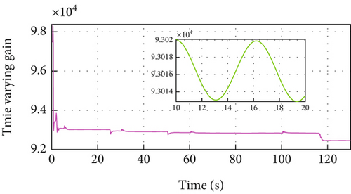
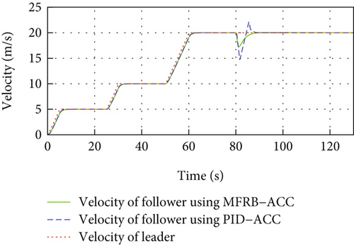
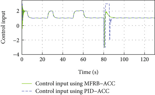
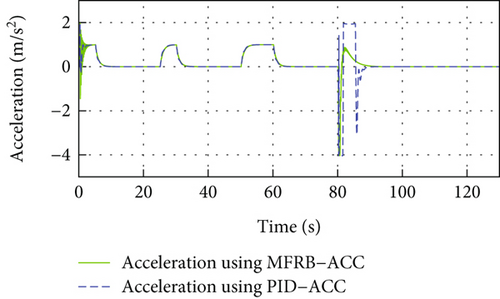
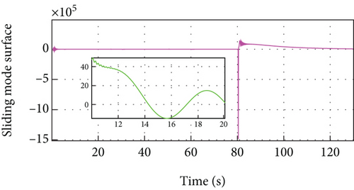
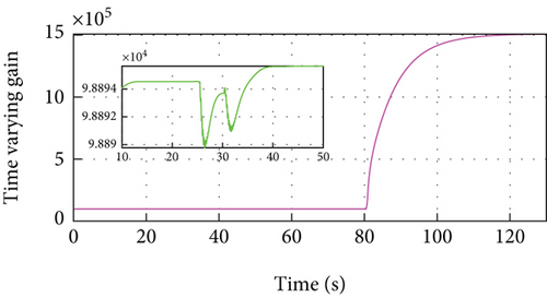
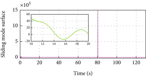
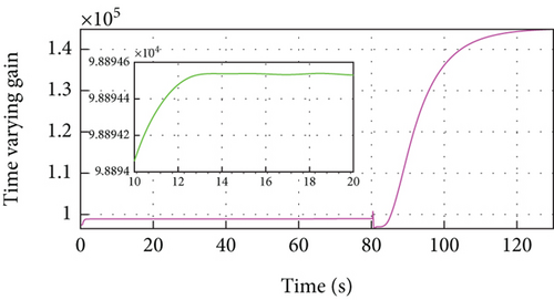
In Figure 8(a), a vehicle cuts between the follower vehicle and the leader vehicle at 80 s, and the developed MFRB-ACC adjusts the distance to the desired distance within 5 s and converges to the desired distance with a small position tracking error within 40 s. However, as shown in Figure 5(a), PID-ACC scheme tracks its preceding vehicle with a larger position tracking error even if it can rapidly adjust the distance to the desired distance. In Figure 8(b), the deviation of speed using PID-ACC is larger than using MFRB-ACC. The velocity curve has overshoot using PID-ACC. The change of speed is smooth using MFRB-ACC. All of these illustrate that MFRB-ACC leads to better ride comfort than PID-ACC. In addition, it can also demonstrate that the MFRB-ACC has strong robustness in different work conditions. These results can be also demonstrated in Figures 8(c) and 8(d). The PID-ACC leads to input saturation and leads to the vehicle moving with maximum acceleration and deceleration. However, the control input and acceleration using MFRB-ACC are smooth. Figures 8(e) and 8(f) show the sliding mode surface and time-varying gain.

4.3.2. Cut-Out Condition

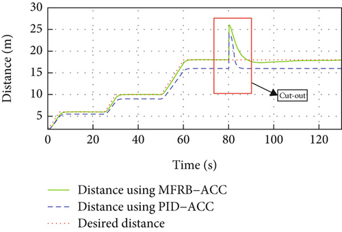
As shown in Figure 7(b), in this condition, the leader vehicle cuts out the current lane, and the follower vehicle remarks the leader vehicle. As a result, the distance between the follower vehicle and the new leader vehicle is larger than the desired distance. Same as Section 4.3.1, this simulation is based on the example in Section 4.2.1, and we assume that the leader vehicle cuts out the current lane at 80 s, and the distance between the follower vehicle and the new leader vehicle increased by 8 m.

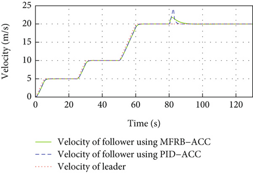
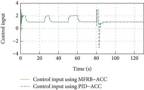
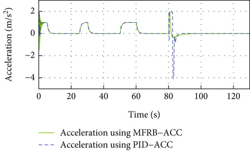
In Figure 9(a), PID-ACC scheme tracks its preceding vehicle with a larger position tracking error even if it can rapidly adjust the distance to the desired distance. MFRB-ACC adjusts the distance to the desired distance asymptotically. As shown in Figure 8(b) and Figure 9(b), the deviation of speed using PID-ACC is also larger than using MFRB-ACC. In Figures 9(c) and 9(d), PID-ACC leads to input saturation and leads to the vehicle moving with maximum acceleration and deceleration. However, the control input and acceleration using MFRB-ACC are smooth. Figures 9(e) and 9(f) show the sliding mode surface and time-varying gain. All of these show the advantages of MFRB-ACC in tracking performance and robustness.

5. Conclusion

(i)
This paper has studied the ACC problem of the nonlinear vehicle with disturbances. A novel MFRB-ACC method including PI control, feedback control, and robust control was designed. The model information was completely removed, and robust cruising control was ensured for the vehicle only using position and velocity data
(ii)
The designed MFRB-ACC algorithm can accurately achieve different spacing targets such as CTH and VTH. Theoretically, this algorithm can accurately achieve any spacing policy
(iii)
The designed MFRB-ACC can effectively compensate the discrete error caused by the low sampling frequency. Whether the sampling time is 0.01 s or 0.1 s, the designed MFRB-ACC algorithm can accurately track the leader vehicle with the desired distance
(iv)
The designed MFRB-ACC has strong robustness. It can achieve stable and safe distance adjustment in different conditions, such as cut-in and cut-out

The designed MFRB-ACC can be applied to many nonlinear systems that are difficult to accurately model, such as robots, UAVs, and unmanned ships. Like many existing robust control methods, the designed controller has discontinuous robust term causing chatting phenomena, cannot be applied to or cannot be directly used on hardware platforms, and needs to be matched with other power electronics technologies. In the future, under the control framework of this paper, research on ACC control such as chatting-free will be carried out, and a comprehensive physical platform will be established.

Conflicts of Interest

The authors declare that there is no conflict of interest regarding the publication of this paper.

Acknowledgments

This work was supported by the Fundamental Research Funds for the Central University of China, Grant/Award number: Z1090122053.

Open Research

Data Availability

The data used to support the findings of this study are included within the article.

References

1 Wang K. and Chaoxu M., Learning-based control with decentralized dynamic event-triggering for vehicle systems, IEEE Transactions on Industrial Informatics. (2023) 19, no. 3, 2629–2639, https://doi.org/10.1109/TII.2022.3168034.
10.1109/TII.2022.3168034
Web of Science® Google Scholar
2 Khound P., Will P., and Gronwald F., Design methodology to derive over-damped string stable adaptive cruise control systems, IEEE Transactions on Intelligent Vehicles. (2022) 7, no. 1, 32–44, https://doi.org/10.1109/TIV.2021.3066056.
10.1109/TIV.2021.3066056
Google Scholar
3 Li T., Chen D., Zhou H., Laval J., and Xie Y., Car-following behavior characteristics of adaptive cruise control vehicles based on empirical experiments, Transportation Research Part B: Methodological. (2021) 147, 67–91, https://doi.org/10.1016/j.trb.2021.03.003.
10.1016/j.trb.2021.03.003
Web of Science® Google Scholar
4 Huang Z., Chu D., Chaozhong W., and He Y., Path planning and cooperative control for automated vehicle platoon using hybrid automata, IEEE Transactions on Intelligent Transportation Systems. (2019) 20, no. 3, 959–974, https://doi.org/10.1109/TITS.2018.2841967, 2-s2.0-85049984015.
10.1109/TITS.2018.2841967
Web of Science® Google Scholar
5 Kural E. and Güvenç B. A., Model predictive adaptive cruise control, 2010 IEEE International Conference on Systems, Man and Cybernetics, 2010, Istanbul, Turkey, 1455–1461, https://doi.org/10.1109/ICSMC.2010.5642478, 2-s2.0-78751472162.
10.1109/ICSMC.2010.5642478
Google Scholar
6 Li S., Li K., Rajamani R., and Wang J., Model predictive multi-objective vehicular adaptive cruise control, IEEE Transactions on Control Systems Technology. (2011) 19, no. 3, 556–566, https://doi.org/10.1109/TCST.2010.2049203, 2-s2.0-79955483508.
10.1109/TCST.2010.2049203
PubMed Web of Science® Google Scholar
7 Zhao D. and Wang B., Data-based vehicle adaptive cruise control: a review, Proceedings of the 32nd Chinese Control Conference, 2013, Xi′an, China, 7840–7845.
Google Scholar
8 Yan M., Song J., Yang P., and Tang Y., Distributed adaptive sliding mode control for vehicle platoon with uncertain driving resistance, 2017 36th Chinese Control Conference (CCC), 2017, Dalian, China, 9396–9400, https://doi.org/10.23919/ChiCC.2017.8028855, 2-s2.0-85032201580.
10.23919/ChiCC.2017.8028855
Google Scholar
9 Yan M., Song J., Yang P., and Zuo L., Neural adaptive sliding-mode control of a bidirectional vehicle platoon with velocity constraints and input saturation, Complexity. (2018) 2018, 11, https://doi.org/10.1155/2018/1696851, 2-s2.0-85062700664, 1696851.
10.1155/2018/1696851
Google Scholar
10 Weng Y. and Gao X., Adaptive sliding mode decoupling control with data-driven sliding surface for unknown mimo nonlinear discrete systems, Circuits, Systems, and Signal Processing. (2017) 36, no. 3, 969–997, https://doi.org/10.1007/s00034-016-0353-0, 2-s2.0-85012964679.
10.1007/s00034-016-0353-0
Web of Science® Google Scholar
11 Gao S., Hou Y., Dong H., Yue Y., and Li S., Global nested PID control of strict-feedback nonlinear systems with prescribed output and virtual tracking performance, IEEE Transactions on Circuits and Systems II: Express Briefs. (2020) 67, no. 2, 325–329, https://doi.org/10.1109/TCSII.2019.2907141.
10.1109/TCSII.2019.2907141
Web of Science® Google Scholar
12 Milanés V., Villagrá J., Godoy J., and González C., Comparing fuzzy and intelligent PI controllers in stop-and-go manoeuvres, IEEE Transactions on Control Systems Technology. (2012) 20, no. 3, 770–778, https://doi.org/10.1109/TCST.2011.2135859, 2-s2.0-84859882641.
10.1109/TCST.2011.2135859
Web of Science® Google Scholar
13 Lidström K., Sjöberg K., Holmberg U., Andersson J., Bergh F., Bjäde M., and Mak S., A modular CACC system integration and design, IEEE Transactions on Intelligent Transportation Systems. (2012) 13, no. 3, 1050–1061, https://doi.org/10.1109/TITS.2012.2204877.
10.1109/TITS.2012.2204877
Web of Science® Google Scholar
14 Li S. E., Zheng Y., Li K., and Wang J., An overview of vehicular platoon control under the four-component framework, 2015 IEEE Intelligent Vehicles Symposium (IV), 2015, Seoul, Korea, 286–291, https://doi.org/10.1109/IVS.2015.7225700, 2-s2.0-84951041958.
10.1109/IVS.2015.7225700
Google Scholar
15 Nieuwenhuijze M. R. I., van Keulen T., Öncü S., Bonsen B., and Nijmeijer H., Cooperative driving with a heavy-duty truck in mixed traffic: experimental results, IEEE Transactions on Intelligent Transportation Systems. (2012) 13, no. 3, 1026–1032, https://doi.org/10.1109/TITS.2012.2202230.
10.1109/TITS.2012.2202230
Web of Science® Google Scholar
16 Lin T.-W., Hwang S.-L., and Green P. A., Effects of time-gap settings of adaptive cruise control (ACC) on driving performance and subjective acceptance in a bus driving simulator, Safety Science. (2009) 47, no. 5, 620–625, https://doi.org/10.1016/j.ssci.2008.08.004, 2-s2.0-61549124104.
10.1016/j.ssci.2008.08.004
Web of Science® Google Scholar
17 Chiang Y.-H. and Juang J.-C., Longitudinal vehicle control with the spacing policy in consideration of brake input limits, 2007 IEEE International Conference on Systems, Man and Cybernetics, 2007, Montreal, QC, Canada, 1705–1710, https://doi.org/10.1109/ICSMC.2007.4413810, 2-s2.0-40949124300.
10.1109/ICSMC.2007.4413810
Google Scholar
18 Zhou J. and Peng H., Range policy of adaptive cruise control vehicles for improved flow stability and string stability, IEEE Transactions on Intelligent Transportation Systems. (2005) 6, no. 2, 229–237, https://doi.org/10.1109/TITS.2005.848359, 2-s2.0-21644459284.
10.1109/TITS.2005.848359
Web of Science® Google Scholar
19 Zhang J. and Ioannou P. A., Adaptive vehicle following control system with variable time headways, Proceedings of the 44th IEEE Conference on Decision and Control, 2005, Seville, Spain, 3880–3885, https://doi.org/10.1109/CDC.2005.1582767, 2-s2.0-33745194247.
10.1109/CDC.2005.1582767
Google Scholar
20 Ahmad E., Iqbal J., Khan M. A., Liang W., and Youn I., Predictive control using active aerodynamic surfaces to improve ride quality of a vehicle, Electronics. (2020) 9, no. 9, https://doi.org/10.3390/electronics9091463.
10.3390/electronics9091463
PubMed Web of Science® Google Scholar
21 Shakouri P. and Ordys A., Nonlinear model predictive control approach in design of adaptive cruise control with automated switching to cruise control, Control Engineering Practice. (2014) 26, 160–177, https://doi.org/10.1016/j.conengprac.2014.01.016, 2-s2.0-84897741187.
10.1016/j.conengprac.2014.01.016
Web of Science® Google Scholar
22 Zhang H., Liang J., and Zhang Z., Active fault tolerant control of adaptive cruise control system considering vehicle-borne millimeter wave radar sensor failure, IEEE Access. (2020) 8, 11228–11240, https://doi.org/10.1109/ACCESS.2020.2964947.
10.1109/ACCESS.2020.2964947
Web of Science® Google Scholar
23 Song J., Yan M., Yongfeng J., and Yang P., Nonlinear gain feedback adaptive DSC for a class of uncertain nonlinear systems with asymptotic output tracking, Nonlinear Dynamics. (2019) 98, no. 3, 2195–2210, https://doi.org/10.1007/s11071-019-05317-7.
10.1007/s11071-019-05317-7
Web of Science® Google Scholar
24 Lin Y.-C., Nguyen H.-L. T., and Wang C.-H., Adaptive neuro-fuzzy predictive control for design of adaptive cruise control system, 2017 IEEE 14th International Conference on Networking, Sensing and Control (ICNSC), 2017, Calabria, 767–772, https://doi.org/10.1109/ICNSC.2017.8000187, 2-s2.0-85028503628.
10.1109/ICNSC.2017.8000187
Google Scholar
25 Weng Y. and Wang N., Data-driven robust backstepping control of unmanned surface vehicles, International Journal of Robust and Nonlinear Control. (2020) 30, no. 9, 3624–3638, https://doi.org/10.1002/rnc.4956.
10.1002/rnc.4956
Web of Science® Google Scholar
26 Xuhui B., Zhu P., Hou Z., and Liang J., Finite-time consensus for linear multi-agent systems using data-driven terminal ILC, IEEE Transactions on Circuits and Systems II: Express Briefs. (2020) 67, no. 10, 2029–2033, https://doi.org/10.1109/TCSII.2019.2944409.
10.1109/TCSII.2019.2944409
Web of Science® Google Scholar
27 Zhang Y. and Song J., Nonlinear leader-following mass control: a data-driven adaptive sliding mode approach with prescribed performance, Nonlinear Dynamics. (2022) 108, no. 1, 349–361, https://doi.org/10.1007/s11071-022-07218-8.
10.1007/s11071-022-07218-8
Web of Science® Google Scholar
28 Afifa R., Ali S., Pervaiz M., and Iqbal J., Adaptive backstepping integral sliding mode control of a mimo separately excited DC motor, Robotics. (2023) 12, no. 4, https://doi.org/10.3390/robotics12040105.
10.3390/robotics12040105
Web of Science® Google Scholar
29 Cho M. G., Jung U., An J.-Y., Choi Y.-S., and Kim C.-J., Adaptive trajectory tracking control for rotorcraft using incremental backstepping sliding mode control strategy, International Journal of Aerospace Engineering. (2021) 2021, 15, https://doi.org/10.1155/2021/4945642, 4945642.
10.1155/2021/4945642
Web of Science® Google Scholar
30 Li Y., Liu Y., and Tong S., Observer-based neuro-adaptive optimized control of strict-feedback nonlinear systems with state constraints, IEEE Transactions on Neural Networks and Learning Systems. (2022) 33, no. 7, 3131–3145, https://doi.org/10.1109/TNNLS.2021.3051030, 33497342.
10.1109/TNNLS.2021.3051030
PubMed Web of Science® Google Scholar
31 Luo C., Lei H., Zhang D., and Zou X., Adaptive neural control of hypersonic vehicles with actuator constraints, International Journal of Aerospace Engineering. (2018) 2018, 15, https://doi.org/10.1155/2018/1284753, 2-s2.0-85059101356, 1284753.
10.1155/2018/1284753
Web of Science® Google Scholar
32 Liu L., Zhao W., Liu Y.-J., Tong S., and Wang Y.-Y., Adaptive finite-time neural network control of nonlinear systems with multiple objective constraints and application to electromechanical system, IEEE Transactions on Neural Networks and Learning Systems. (2021) 32, no. 12, 5416–5426, https://doi.org/10.1109/TNNLS.2020.3027689, 33064656.
10.1109/TNNLS.2020.3027689
PubMed Web of Science® Google Scholar
33 Zhou W., Jun F., Yan H., Xin D., Wang Y., and Zhou H., Event-triggered approximate optimal path-following control for unmanned surface vehicles with state constraints, IEEE Transactions on Neural Networks and Learning Systems. (2023) 34, no. 1, 104–118, https://doi.org/10.1109/TNNLS.2021.3090054, 34224359.
10.1109/TNNLS.2021.3090054
PubMed Web of Science® Google Scholar
34 Yuan X., Chen B., and Lin C., Prescribed finite-time adaptive neural tracking control for nonlinear state-constrained systems: barrier function approach, IEEE Transactions on Neural Networks and Learning Systems. (2022) 33, no. 12, 7513–7522, https://doi.org/10.1109/TNNLS.2021.3085324.
10.1109/TNNLS.2021.3085324
PubMed Web of Science® Google Scholar
35 Liu S., Wang Y., Li Y., Yan B., and Zhang T., Cooperative guidance for active defence based on line-of-sight constraint under a low-speed ratio, The Aeronautical Journal. (2023) 127, no. 1309, 491–509, https://doi.org/10.1017/aer.2022.62.
10.1017/aer.2022.62
Web of Science® Google Scholar
36 Liu S., Yan B., Zhang T., Dai P., Liu R., and Yan J., Three-dimensional cooperative guidance law for intercepting hypersonic targets, Aerospace Science and Technology. (2022) 129, article 107815, https://doi.org/10.1016/j.ast.2022.107815.
10.1016/j.ast.2022.107815
Web of Science® Google Scholar
37 Liu S., Yan B., Zhang T., Dai P., and Yan J., Guidance law with desired impact time and FOV constrained for antiship missiles based on equivalent sliding mode control, International Journal of Aerospace Engineering. (2021) 2021, 15, https://doi.org/10.1155/2021/9923332, 9923332.
10.1155/2021/9923332
Web of Science® Google Scholar
38 Liu S., Binbin Yan X., Zhang W. L., and Yan J., Fractional-order sliding mode guidance law for intercepting hypersonic vehicles, Aerospace. (2022) 9, no. 2, https://doi.org/10.3390/aerospace9020053.
10.3390/aerospace9020053
Web of Science® Google Scholar
39 Rsetam K., Cao Z., Wang L., Al-Rawi M., and Man Z., Practically robust fixed-time convergent sliding mode control for underactuated aerial flexible jointrobots manipulators, Drones. (2022) 6, no. 12, https://doi.org/10.3390/drones6120428.
10.3390/drones6120428
Google Scholar
40 Khan R. F. A., Rsetam K., Cao Z., and Man Z., Singular perturbation-based adaptive integral sliding mode control for flexible joint robots, IEEE Transactions on Industrial Electronics. (2023) 70, no. 10, 10516–10525, https://doi.org/10.1109/TIE.2022.3222684.
10.1109/TIE.2022.3222684
Web of Science® Google Scholar
41 Rsetam K., Cao Z., and Man Z., Design of robust terminal sliding mode control for underactuated flexible joint robot, IEEE Transactions on Systems, Man, and Cybernetics: Systems. (2022) 52, no. 7, 4272–4285, https://doi.org/10.1109/TSMC.2021.3096835.
10.1109/TSMC.2021.3096835
Web of Science® Google Scholar
42 Rsetam K., Cao Z., and Man Z., Cascaded-extended-state-observer-based sliding-mode control for underactuated flexible joint robot, IEEE Transactions on Industrial Electronics. (2020) 67, no. 12, 10822–10832.
10.1109/TIE.2019.2958283
Web of Science® Google Scholar
43 Mehmood Y., Aslam J., Ullah N., Alsheikhy A. A., Din E. U., and Iqbal J., Robust fuzzy sliding mode controller for a skid-steered vehicle subjected to friction variations, PLoS One. (2021) 16, no. 11, article e0258909, https://doi.org/10.1371/journal.pone.0258909, 34784368.
10.1371/journal.pone.0258909
PubMed Web of Science® Google Scholar
44 Ahmad S., Uppal A. A., Azam M. R., and Iqbal J., Chattering free sliding mode control and state dependent Kalman filter design for underground gasification energy conversion process, Electronics. (2023) 12, no. 4, https://doi.org/10.3390/electronics12040876.
10.3390/electronics12040876
Web of Science® Google Scholar
45 Wang Z. and Zhao T., Based on robust sliding mode and linear active disturbance rejection control for attitude of quadrotor load UAV, Nonlinear Dynamics. (2022) 108, no. 4, 3485–3503, https://doi.org/10.1007/s11071-022-07349-y.
10.1007/s11071-022-07349-y
Web of Science® Google Scholar

Citing Literature

All articles

Model-Free Robust Backstepping Adaptive Cruise Control

Abstract

1. Introduction

1.1. ACC from Vehicle Model Perspective

1.2. ACC from Spacing Strategy Perspective

1.3. ACC from Control Method Perspective

2. Problem Formulation

2.1. Vehicle Motion with Disturbances

2.2. The Adaptive Cruise Objective

3. Adaptive Cruise Control Design

3.1. Backstepping Error

3.2. Model-Free Vehicle System Description: Data-Driven Sliding Surface

3.3. Robust Controller

3.4. Stability Analysis

4. Simulation Studies

4.1. Validation of Control Performance for the Spacing Strategy

4.1.1. Control Performance for CTH

4.1.2. Control Performance for VTH

4.2. Validation of Control Performance for the Sampling Time

4.2.1. Control Performance for CTH

4.2.2. Control Performance for VTH

4.3. Validation of Control Performance for Typical Condition

4.3.1. Cut-In Condition

4.3.2. Cut-Out Condition

5. Conclusion

Conflicts of Interest

Acknowledgments

Open Research

Data Availability

References

Citing Literature

Figures

References

Information

About Wiley Online Library

Help & Support

Opportunities

Connect with Wiley

Model-Free Robust Backstepping Adaptive Cruise Control

Abstract

1. Introduction

1.1. ACC from Vehicle Model Perspective

1.2. ACC from Spacing Strategy Perspective

1.3. ACC from Control Method Perspective

2. Problem Formulation

2.1. Vehicle Motion with Disturbances

2.2. The Adaptive Cruise Objective

3. Adaptive Cruise Control Design

3.1. Backstepping Error

3.2. Model-Free Vehicle System Description: Data-Driven Sliding Surface

3.3. Robust Controller

3.4. Stability Analysis

4. Simulation Studies

4.1. Validation of Control Performance for the Spacing Strategy

4.1.1. Control Performance for CTH

4.1.2. Control Performance for VTH

4.2. Validation of Control Performance for the Sampling Time

4.2.1. Control Performance for CTH

4.2.2. Control Performance for VTH

4.3. Validation of Control Performance for Typical Condition

4.3.1. Cut-In Condition

4.3.2. Cut-Out Condition

5. Conclusion

Conflicts of Interest

Acknowledgments

Open Research

Data Availability

References

Citing Literature

Figures

References

Related

Information