Lane-Changing Trajectory Prediction Modeling Using Neural Networks
Abstract
Concerning autonomous driving, lane-changing (LC) is essential, particularly within complicated dynamic settings. It is a challenging task to model LC since driving behavior is complicated and uncertain. The present study adopts a dual-layer feed-forward backpropagation neural network involving sigmoid hidden neurons and linear output neurons for evaluating intrinsic LC complexity. Furthermore, the estimation and validation of the model were performed by large-scale trajectory data. Empirical LC data were obtained from the Next Generation Simulation (NGSIM) project for training and testing the neural network-based LC model. The findings revealed that the introduced model could make precise LC predictions of vehicles under small trajectory errors and satisfactory accuracy. The present work assessed LC beginning/endpoints and velocity estimates by analyzing the vehicles around. It was observed that the neural network model yielded almost the same predictions as the observational LC trajectories as well as following vehicle trajectories on the original and target lanes. Furthermore, for LC behavior characteristic validation, the neural network-produced LC gap distributions underwent comparisons to real-life data, demonstrating the characteristics of LC gap distributions not to differ from the real-life LC behavior substantially. Eventually, the introduced neural network-based LC model was compared to a support vector regression-based LC model. It was found that the trajectory predictions of both models were adequately consistent with the observational data and could capture both lateral and longitudinal vehicle movements. In turn, this demonstrates that the neural network and support vector regression models had satisfactory performance. Also, the proposed models were evaluated using new inputs such as speed, gap, and position of the subject vehicle. The analysis findings indicated that the performance of the proposed NN and SVR models was higher than the model with new inputs.
1. Introduction
It is expected that an interconnected environment contributes to the solving of a large number of transportation problems in association with mobility, efficiency, environmental impacts, and safety. Connected environments help drivers navigate the current and future driving conditions, particularly information on likely but unobserved hazards. Consequently, drivers can make lane-changing (LC) decisions at higher safety and information levels within connected environments [1]. Carelessly performed LC could be a hazardous maneuver. LC is a complicated driving process, for which it is required to match the speed in the present lane with speed in the target lane and identify a proper gap within the greatest lane to ensure the LC intention recognition of the driver by the other drivers and good LC [2]. The LC and car-following (CF) models in traffic flow theory perform lateral and longitudinal interaction analyses while driving before the detailed description of LC and CF behavior. The CF model has been long and extensively studied. In comparison to the CF state, the pressure and workload of drivers are substantially enhanced in an LC process, exposing the driver to a high level of hazard and error [3–6]. Several studies presented empirical evidence proposing LC and CF behaviors to be majorly responsible for oscillation formation and enhancement on freeways with multiple lanes [7–9]. Typically, traveling speed heterogeneity between various lanes triggers the LC maneuvers of vehicles. LC behavior is involved in traffic congestion. LC occurring at the onset of congestion might reduce the traffic capacity on account of undesirable LC behavior, inducing and propagating stop-go shockwaves. Earlier works demonstrated LC to induce frequent changes in the speeds and gaps on the original and target lanes. A complete lane-changing decision (CLACD) modeling framework that explains both the mandatory and discretionary lane-changing behaviors is developed. An integrated approach is employed to model discretionary lane-changing behavior by combining the target lane selection using the utility theory approach and the gap acceptance behavior using a game theory approach. Results reveal that the CLACD models can effectively capture the observed DLC decisions with high accuracy. Furthermore, the CLACD model shows a realistic prediction of traffic flow patterns compared with the utility theory model [10]. This would add to the likelihood of collisions [11–14], disturbance in traffic flow [15, 16], and reduced capacity [17–19]. Compared to CF behavior investigation, the study of LC behavior requires a larger amount of data for support. Considering such negative LC effects on the safety and flow of traffic, it remains an interesting context to model LC behavior. LC modeling has recently been of higher interest to researchers since the fabrication of connected automated vehicles (CAVs) enables the easy acquisition of many datasets through advanced sensing devices. Furthermore, it is possible to transmit regular data (including velocity, position, directly-unobtainable data such as the steering angle, vehicle mass, and acceleration) among vehicles, between vehicles to road identities, and from vehicles to the cloud technology [20]. In general, one can classify LC into LC decisions (LCD) and LC implementation (LCI). In the former, drivers have mental motivation for changing lanes based on the around traffic, while the latter refers to a physical procedure, in which vehicles move from a lane to a target one [21]. It is possible to predict LC, such as any driving behavior predictions, in a classification or regression problem. The former case is aimed at vehicle state discretization to allow quicker real-time vehicle behavior distinguishing, while the latter case seeks to make speed and position predictions for vehicle road movement mapping [22, 23]. Concerning self-driving vehicles, four phases exist, i.e., (1) environment perception, (2) information processing, (3) the behavior prediction of others in the same environment, and (4) driving decision-making [24]. A driver often needs to respond to a lane-changing request of a lane-changer, which is a function of their personality traits and the current driving conditions. Drivers’ responses to lane-changing requests were examined in a connected environment using the CARRS-Q Advanced Driving Simulator. Additionally, drivers’ response times are modeled using a random parameter accelerated failure time (AFT) hazard-based duration model. Results revealed that drivers tend to be more cooperative in response to a lane-changing request in the connected environment compared with the baseline condition whereby they tend to accelerate to avoid the lane-changing request [25]. Hence, a large number of works were conducted to focus on the two-dimensional prediction of trajectories for the driving behavior mimicking of humans [26–30]. LC modeling is among the most prominent areas of transportation-related study. Thus, earlier works developed some LC models in recent decades. These models may be classified into two groups: (1) analytical and (2) data-driven models. There are a relatively small number of data-driven and analytical works. This could be attributed to difficult LCI data collection at a large scale [31–34]. Also, earlier works proved that data-driven models outperformed conventional analytical ones in several characteristics, e.g., trajectory accuracy and traffic flow characteristic replication [35–39]. Such studies adopted the neural network (NN) approach in several variants. Generally, the driving behavior of humans is of high degrees of nonlinearity and complexity. Thus, it cannot be easily modeled using conventional shallow machine learning or mathematical approaches [40]. Despite the introduction of some LC models, numerous questions are yet to be answered to realize LC behavior. For instance, analytical LC models obtain an accuracy of 70–80% in prediction [41]. Also, a significant degree of inconsistency exists between observations and modeled principles [42]. Indeed, it is expected that models of higher accuracy are developed. A small number of studies with careful examination of LCI can be found. An analytical model cannot easily and accurately consider LC uncertainty and diversity [32, 43, 44]. On the other hand, a data-driven model can solely consider influential factors at a particular time [31]. The historical data shortly before the rapid movement of a driver is an essential component [45]. Data-driven and analytical models mostly take into account LCD or LCI separately. This may not lead to complete LC process reproduction consisting of LCI and LCD and their influence on the traffic behavior.
NNs have enjoyed the highest popularity in data-driven LCI and LCD works. Such popularity arises from (1) their capability of dealing with noisy data estimating unlimited complexity extents under nonlinearity and (2) their need for no simplification or prior awareness of solving the problem, unlike statistical approaches [46]. Hunt and Lyons [47] modeled dual carriageway LCD through the BP-NN approach. Their model estimated LCD on the grounds of the busy traffic in the adjacency. They exploited empirical traffic data and simulation results to demonstrate the competence of their model. Li et al. [48] studied LCD prediction using NN and BF. They incorporated steering wheel angle, and lane line sensor parameters along with in-vehicle CAN bus acquisition characteristics. Comparison of the results to empirical data revealed an accuracy of up to 91.38%. Ke and Wang [49] introduced an LCD approach for the training and learning of connected automated vehicles (CAVs). Their approach included a microscale cellular automata-based simulation model and a BP-NN model, which could make rapid decisions on whether to perform an LC maneuver or keep the lane. Their approach was found to be efficient in the LCD prediction of CAVs. Compared to data-driven LCD approaches, a small number of works were identified to have conducted NN-based LCI investigations. Ding et al. [31] studied real-time LC trajectory prediction by using a dual-layer feed-forward BP-NN approach. The review of earlier works suggested that the BP-NN model was valid for LCD and LCI.
To deal with the barriers of LC modeling, the present work adopts a dual-layer feed-forward backpropagation NN that contains hidden sigmoid neurons and linear output neurons for evaluating the intrinsic LC complexity. Furthermore, the model is estimated and validated using trajectory data at a large scale. The NN may automatically identify essential characteristics that affect the entire LC process by solely observing position data of four vehicles around the intended vehicle, predicting vehicles’ behavior. This study mainly seems to develop a neural network approach for LC prediction based on vehicle position data. Empirical vehicle trajectories of the next generation simulation (NGSIM) project were exploited to derive delicate LC data. The NN model is trained, tested, and compared to the field data.
The remainder of the present article is organized as follows: Section 2 reviews the LC modeling literature; Section 3 addresses the research gap and highlights the contributions of the present work; Section 4 represents the examination sites and processed data; Section 5 introduces an NN model before introducing the inputs and outputs; Section 6 provides a detailed assessment of the introduced models through empirical data of LC; and Section 7 concludes the study.
2. Literature Review
LC has recently been as interesting as CF; however, a small number of studies can be found on LC in the literature [50]. A large rate of advancements was seen in connected, autonomous vehicles [51, 52] and enhanced insights into the impacts of LC on traffic operations, e.g., traffic build-up, safety, and emissions [53] necessary to construct models with larger advancements. A review of the available LC approaches suggests that LC trajectory estimation has a high improvement potential. In general, LC maneuvers are divided into mandatory and discretionary LC. The former refers to LC required to achieve a predefined route (on account of diverging, merging, or a lane drop, for example), while the latter refers to pursuing LC speed advantages or driving comfort. Most of such models focus on LC intention and circumstances. They believed LC behavior to occur when LC conditions were judged based on the LC intention. They majorly focused on three safe distance components, including (1) the distance from the leading vehicle of the target lane, (2) the distance from the following vehicle of the target lane, and (3) the distance from the leading vehicle of the current lane. Mahajan et al. [54] proposed an end-to-end machine learning framework to make LC maneuver predictions using unlabeled data and a small number of characteristics. They employed density-based clusters for the identification of LC and lane-keeping maneuvers. Then, they trained a support vector machine (SVM) for learning clustered label boundaries and the automatic labeling of new raw datasets. Subsequently, they introduced the labeled data to a long short-term memory (LSTM) framework for maneuver category prediction. Xie et al. [55] modeled in data-driven settings by using deep learning techniques. They applied an LSTM NN and a deep belief network (DBN) for LC modeling by incorporating LCI and LCD. Their data-driven model was found to be capable of accurate vehicle LC prediction. A sensitivity analysis was performed, indicating the relative leading vehicle position on the target lane to be the most prominent LC-related factor. Lee et al. [56] introduced an integrated multilane stochastic continuous car-following framework. They exploited deep learning for the likelihood estimation of LC maneuvers. Particularly, they introduced an LC maneuver-derived stochastic volatility within a multilane stochastic optimal velocity model (SOVM). Furthermore, they employed a convolutional NN (CNN) for LC maneuver likelihood estimation in their integrated stochastic continuous car-following framework. The findings revealed that the integrated SOVM yielded almost the same predictions as the LC trajectory observations and the following vehicles’ trajectories on both the original and target lanes. Zhang et al. [40] employed deep learning and LSTM NN for the simultaneous modeling of LC and CF behaviors. Also, a hybrid retraining constrained (HRC) technique was introduced for further LSTM optimization. The HRC-LSTM model was observed to be capable of accurate LC and CF behavior estimation at the same time under small longitudinal trajectory errors and significant accuracy of LC prediction in comparison to classical techniques.
A review of data-driven LC researches indicates that NNs have been the most exciting instruments. For instance, Tomar et al. [57] adopted a multilayer perceptron (MLP) and introduced an accurate LC trajectory prediction of discrete paths. The MLP was a simple model with a single input, a single hidden layer, and a single output. It was employed to train, test, and predict vehicle trajectories. A detailed effectiveness discussion of backpropagation (BP) NNs was provided by Ding et al. [31] concerning LC trajectory prediction through vehicle records. The BP NN was compared to the Elman network model in terms of the accuracy and training time results. According to the test results, the BP NN was capable of accurately predicting the LC behavior of drivers in traffic flow within urban areas. Also, it was verified that the collected data affected vehicle trajectories. Zheng et al. [46] proposed an NN for the complexity evaluation of LC. They exploited trajectory data at a large scale to estimate and validate their model. Also, they employed a multinomial logit (MNL) model, which was most commonly regarded as an LC framework in earlier studies to make comparisons. The NN was found to have a prediction accuracy of 94.58% and 73.33% for the left and right LC samples, respectively, during model estimation. However, the MNL model can correctly predict solely 13.25% of the right LC samples and 3.33% of the left LC samples. Despite the substantial accuracy reduction of the two models in the model’s validation, the NN predictions were still satisfactory. Dou et al. [35] employed an NN coupled with an SVM to develop a model for mandatory LC prediction at the lane drops of highways. They achieved an accuracy of 78% and 94% for merging and nonmerging behaviors via the positions, vehicle gaps, and speed differences as inputs. However, they provided no explicit discussion of the NN structure. Tang et al. [58, 59] introduced an LC prediction framework by using an adaptive fuzzy NN to judge LC circumstances and perform steering angle prediction during LC. They incorporated the visual search and vehicle operation behaviors of drivers, driving circumstances, and the motion states of vehicles to build a prediction index system of left LCs. Peng et al. [60] proposed a BP NN for LC behavior prediction. Their model could make accurate LC behavior predictions of drivers at least 1.5 seconds earlier than the LC.
- (i)
A small number of works were found in the literature on the detailed investigation of LCI. Concerning analytical frameworks, LC uncertainty and diversity cannot be easily taken into account [44]. Concerning data-driven models, earlier works have included solely impact factors at a given time [31].
- (ii)
To model LC, typically, vehicle speeds and gaps in two lanes (i.e., the current lane and the target lane) at a given time are incorporated into the simulation, whereas the LCD of a driver would depend on the previous traffic states and driving behavior history.
- (iii)
Earlier works on LC behavior incorporated a large number of parameters, including the space gap, time gap, speed, and acceleration. However, the vehicle positions in the adjacency of the subject vehicle were exploited as the NN input.
3. Research Gaps and Contributions
Earlier NN studies mostly identified temporal information, explored current states, or performed action detection after its onset. However, they did not carry out the prediction of future states. Such studies employed offline data processing to analyze the behavior of drivers on account of limited data. Also, several studies can perform training and make future position predictions of LC vehicles in specific discrete path sections rather than throughout the LC path [31]. A review of LC-based NN model indicates that prediction of subject vehicle position with position inputs has not been evaluated yet. For instance, neural network for prediction of lane-changing trajectory based on the past vehicle data is introduced, and inputs like speed and gap are used for NN model [31]. A backpropagation neural network model was developed to predict lane-changing behavior. Lane changing intent time window is determined via visual characteristics extraction of rear-view mirrors [60]. A neural network model to capture the complexity of lane changing is developed, and large-scale trajectory data are employed for model estimation and validation [46]. The present study primarily seeks to propose an NN model for the bold prediction of complete vehicle trajectories through LC behavior. The Levenberg-Marquardt BP algorithm is employed for the training of the NN. However, in the case of impaired memory, the present study uses scaled conjugate gradient BP.
- (i)
Proposing an NN model for perfectly incorporating the effects of the surrounding vehicles on an LC (subject) vehicle
- (ii)
Introducing the positions of both the subject and adjacent vehicles as the model input
- (iii)
The NN model is capable of trajectory prediction of LC vehicles while LC is occurring
- (iv)
Real-life high-resolution data of vehicle trajectories are employed to calibrate and validate the model
- (v)
Comparison of the introduced neural network-based LC model with a support vector regression-based LC model
- (vi)
Comparison of proposed models with new input variables
4. LC Trajectory
4.1. Dataset
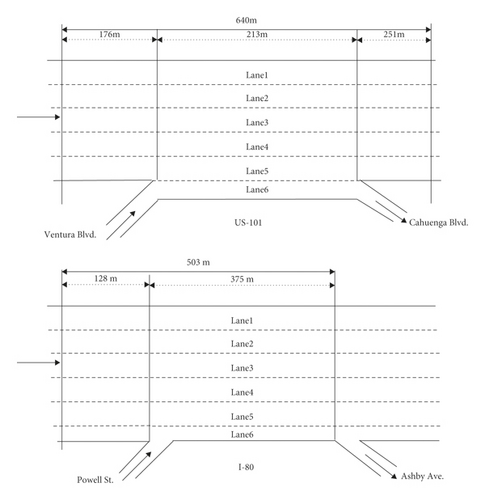
The data of the NGSIM project of FHWA (FHWA, 2008) were exploited in the present work. The NGSIM dataset involves the entire vehicle trajectory dataset of surveillance road sections, i.e., position, acceleration, and speed, at a time interval of 0.1 seconds, along with longitudinal and lateral locations that could be utilized for LC maneuver identification. Three vehicle types, including trucks, cars, and motorcycles, were incorporated. These high-fidelity trajectory data have been extensively utilized in traffic flow research in the recent decade [61–68]. Many LC models have undergone calibration and validation via the NGSIM trajectory dataset [2, 35, 55, 56, 69]. The present work employed the I-80 and US-101 datasets for the construction of LC prediction models. A schematic of the case study sites is demonstrated in Figure 1. As can be seen, an exciting order was applied to perform the left-to-right numbering of lanes. Each of the sites involves an off-ramp and an on-ramp, with expected significant LC activities. In general, LC maneuvers are divided into mandatory and discretionary LC [70]. The present paper incorporated solely cars and selected LC maneuver cases with no following and leading vehicle LC maneuvers relative to an LC vehicle. Due to the discussion of solely discretionary LC, the present work excluded mandatory LC vehicles with on-ramp freeway entering and off-ramp freeway exiting from the trajectory dataset. Furthermore, this study discarded vehicles with more than LC activities or more than one crosses. Consequently, the trajectories of 2000 vehicles (i.e., 400 complete LC vehicles) were derived. This study defined the duration of LC as the required time for continuous lateral LC movement. A summary of the statistical LC duration results of the vehicles is provided in Table 1. According to Table 1, the mean LC duration was calculated to be 6.95 seconds. The LC durations of the vehicles were found to be in the range of 1.6–13.8 seconds. Approximately 95% of the vehicles had an LC duration of shorter than 10 seconds. Hence, the trajectory data of vehicles with an LC duration of below 10 seconds were utilized to eliminate irregular behavior and any noise. Subsequently, the included trajectory dataset involved 100 time-frames (10 s) LC maneuvers on the targeted sections’ entire lanes in the I-80 and US-101 freeways.
| Duration (s) | Total number of vehicles | Proportion (%) |
|---|---|---|
| <2 | 5 | 1.25 |
| 2–4 | 24 | 6 |
| 4–6 | 88 | 22 |
| 6–8 | 179 | 44.75 |
| 8–10 | 79 | 19.75 |
| 10–12 | 19 | 4.75 |
| >12 | 6 | 1.5 |
| Total | 400 | 100 |
4.2. LC Prediction Variables
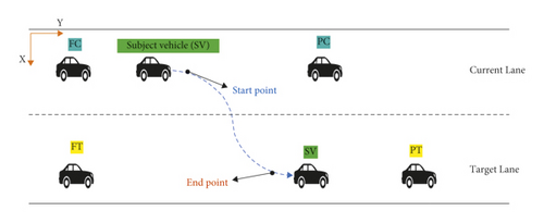
In LC, vehicles perform a two-dimensional planar movement instead of a one-dimensional CF movement. LC maneuvers include several vehicle interactions. It is required to carefully determine the variables that could impact the LC decisions of drivers and LC implementation. In general, an LC model incorporates the acceleration and speed data of vehicles on the neighboring lanes and the leading-lagging vehicle gap on the neighboring lanes. These variables pose various impacts on LC behavior modeling [50, 71]. The extraction of information on two-dimensional lateral and longitudinal positions of adjacent vehicles for predicting the target vehicle position via an NN is a direct LC behavior modeling technique. Therefore, it is possible to extract further and examine the characteristics of LC behavior. To this end, five vehicles, involving the LC one, that were directly associated with a usual LC process were incorporated, as shown in Figure 2. On the original lane, a vehicle (FC) follows the LC vehicle (SV), and another vehicle (PC) is leading. The same definition was applied to the target lane; a vehicle (FT) follows the LC vehicle, and another vehicle (PT) is leading. According to Figure 2, the beginning of LC behavior is considered to be a position in which the heading of the subject vehicle leaves the present lane direction, while the end of LC is a position in which the heading of the subject vehicle converges to the target lane direction.
5. Methodology
5.1. NN Model
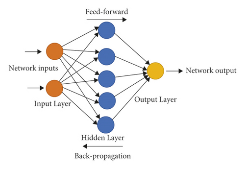
An artificial neural network (ANN) refers to a massive parallel network with simple nonlinear computational components known as neurons. Neurons model several human nervous system functionalities to exploit the human nervous system [72]. ANNs have been often used to approximate nonlinear functions, exhibiting significant benefits for prediction, signal processing, optimization, and pattern identification purposes, in light of their valid and flexible nonlinear self-organization characteristics. ANNs are employed to model a wide range of problems [73–75] and have yielded more significant outcomes than conventional models in several cases. The present work adopted a typical feed-forward BP NN that had sigmoid hidden neurons along with linear output neurons, as shown in Figure 3.
In order to avoid overtraining and overfitting, various datasets were applied to NN training. It was observed that NN had the smallest error when it was trained by 70% of the data, as shown in Figure 4.
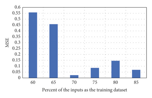
Generally, a rise in the number of hidden layer neurons improves NN estimation accuracy. However, the increased hidden layer neurons would raise the estimation cost and overfitting issue [76]. To bring a more satisfactory trade-off between accuracy and model cost and overfitting, the mean squared error (MSE) is employed to evaluate NNs with different neuron counts in terms of performance, as shown in Figure 4. The present work utilized the Neural Network Toolbox of MATLAB to construct and implement the NN. During learning, 70% of the inputs were employed as the training dataset, while the remaining 30% were exploited as the testing (validation) dataset. This study selected a minimum performance gradient of 10−5. The NN model was trained and tested using a personal computer with a 1.78 GHz CPU. To obtain optimal performance, NN required a computational time of 76 s. The training and testing of NN lasted for 7584 s. Concerning the hidden layer, the minimum MSE was obtained at a neuron count of eight, as shown in Figure 5. Therefore, the number of hidden layer neurons was selected to be eight in the developed model.

5.2. Inputs and Output
It must incorporate historical motions right before the present as LC is a continuous process while driving. The present study focused solely on the two-dimensional prediction of trajectories. Hence, it was required to determine the initial LC states and not distinguishing LC types [77]. Concerning each of the vehicles, the two-dimensional lateral and longitudinal positions of the nearest following and leading vehicles on the present and target lanes were derived through the NGSIM data. The LC model inputs included the time-sequence historical position data of the subject and four adjacent vehicles (Figure 2). Also, the two-dimensional position prediction of the subject vehicle was performed in the following time steps. As mentioned in Subsection 4.1, a total of four hundred complete-LC samples were obtained through the NGSIM data. Two hundred and eighty samples (i.e., 70% of the dataset) were employed as the training dataset, 60 samples (i.e., 15% of the data) were used as the validation dataset, and the remaining 60 samples (15%) were exploited as the testing dataset. Each sample had 10-s LC trajectory data at time intervals of 0.1 seconds. Therefore, each of the samples consisted of a hundred data points. As a result, 28000 and 6000 data points were derived for training and testing, respectively.
Such inputs can ensure the maximum detection flexibility of the subject vehicle by considering implementation for future autonomous vehicles. The LC outputs include the lateral and longitudinal subject vehicle positions in the next time step t + Δt (that is, [yt+Δt and xt+Δt]).
An NN contains a large number of parameters that could impact model performance. Table 2 provides the ultimate parameters.
| Parameter | Value |
|---|---|
| Input dimension | 10 |
| Output dimension | 2 |
| Historical length (0.1 s) | 100 |
| Neurons in the hidden layer | 8 |
| Training function | Levenberg-Marquardt BP |
| Adaption learning function | Gradient descent with momentum weight and bias |
| Activation function | Sigmoid |
| Performance function | MSE |
| Transfer function | Hyperbolic tangent sigmoid |
5.3. Evaluation Indexes of Model Performance
6. Analysis of Results
6.1. NN-Based LC Model Training
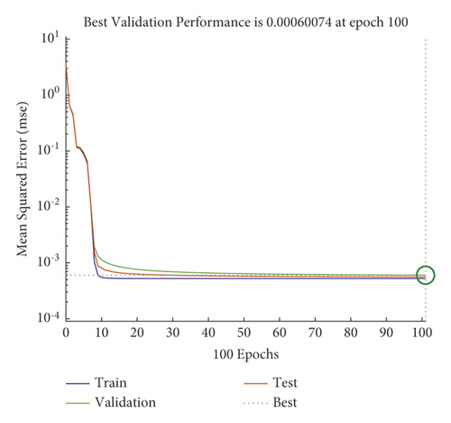
The training convergence rate of NN is depicted in Figure 6. According to Figure 6, MSE underwent a sharp decline as the iterations increased in number. However, a further rise in the number of iterations did not raise the error when the iterations were adequate. Hence, 100 iterations were applied to the NN training phase, fitting the cross-validation criterion.
6.2. NN-Based LC Model Testing
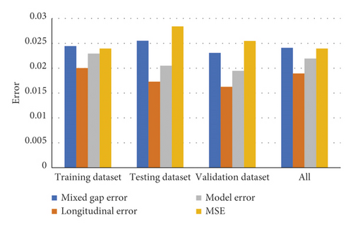
Table 2 reports the training and testing descriptions of the NN-based LC model for performance evaluation. Figure 7 compares the NN model errors by the training, validation, and testing datasets. A comparison of the training and testing datasets demonstrates the overfitting elimination capability of the model. According to Figure 7, the NN model had rationally satisfactory overall predictive accuracy. For instance, the model error of trajectory predictions varied in the range of 0.02. Likewise, the longitudinal and mixed gap errors were found to be reasonable. It should be noted that the validation dataset had lower errors than those of the training and testing data in LC prediction, probably due to the smaller LC variance range of the validation dataset than those of the training and testing datasets.
Numerical tests were performed via the NN-based LC model for the trajectory prediction of sixty test-subjected vehicles. MSE was utilized as the index of performance throughout LC. Table 3 shows LC trajectory prediction MSE values of testing data.
| Vehicle ID | MSE | Vehicle ID | MSE | Vehicle ID | MSE | Vehicle ID | MSE |
|---|---|---|---|---|---|---|---|
| 1 | 0.002856 | 116 | 0.028738 | 227 | 0.038079 | 303 | 0.008232 |
| 5 | 0.038951 | 127 | 0.015417 | 229 | 0.024462 | 305 | 0.010341 |
| 9 | 0.016114 | 132 | 0.032765 | 231 | 0.032455 | 308 | 0.009231 |
| 14 | 0.015715 | 138 | 0.005665 | 235 | 0.013674 | 318 | 0.006383 |
| 17 | 0.016722 | 155 | 0.053034 | 245 | 0.0128 | 332 | 0.009371 |
| 41 | 0.004317 | 169 | 0.005756 | 251 | 0.109571 | 341 | 0.020761 |
| 48 | 0.001693 | 171 | 0.010034 | 261 | 0.032929 | 350 | 0.006996 |
| 67 | 0.016677 | 175 | 0.011424 | 269 | 0.013852 | 353 | 0.073539 |
| 82 | 0.063285 | 191 | 0.021472 | 279 | 0.013526 | 362 | 0.016257 |
| 84 | 0.015718 | 199 | 0.006295 | 283 | 0.026079 | 373 | 0.012606 |
| 89 | 0.016327 | 204 | 0.00577 | 288 | 0.085814 | 378 | 0.019155 |
| 97 | 0.023275 | 206 | 0.010235 | 289 | 0.020792 | 381 | 0.032565 |
| 102 | 0.031238 | 211 | 0.029085 | 293 | 0.351535 | 388 | 0.092071 |
| 111 | 0.007692 | 215 | 0.018323 | 298 | 0.006679 | 393 | 0.011971 |
| 113 | 0.006326 | 218 | 0.00904 | 301 | 0.005626 | 397 | 0.047062 |
Figure 8 depicts the LC trajectory prediction MSE values of twenty vehicles selected randomly (i.e., testing data). The mean MSE value of the tested vehicles was calculated to be nearly 0.0284. As can be seen, MSE is low, suggesting that the developed LC model is capable of adequately capturing the entire LC process. Figure 9 compares trajectory observations and predictions for the twenty randomly selected vehicles. The results suggest the important consistency of the trajectory predictions and observations. Thus, the model could capture both lateral and longitudinal vehicle motions, and the model is demonstrated to perform properly.
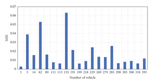
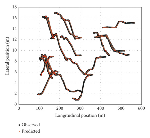
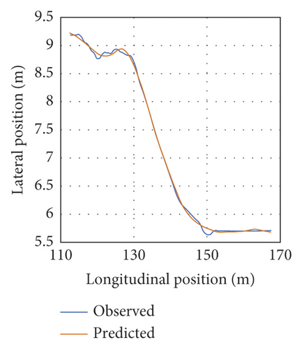
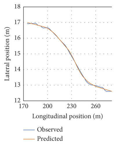
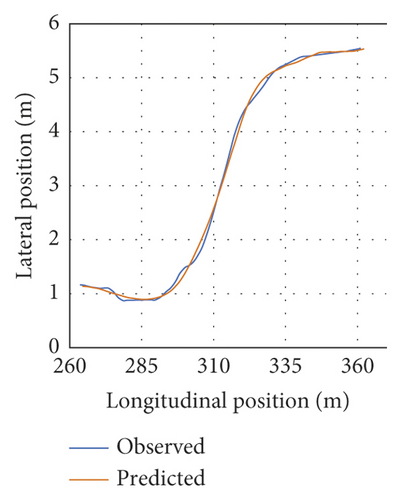
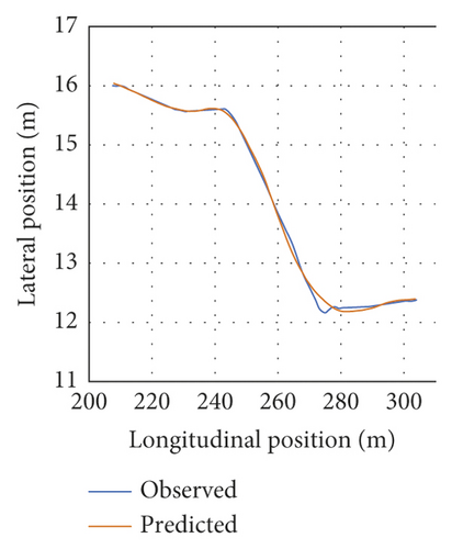
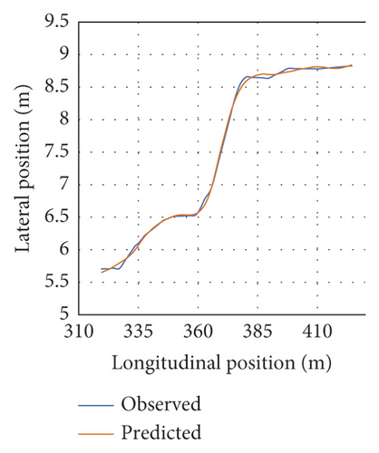
Figure 10 illustrates the LC trajectory predictions and observations of five vehicles. They were selected from the twenty vehicles selected randomly (i.e., testing data). As can be seen, Vehicle 1 had the lowest MSE (Figure 10(a)), whereas Vehicle 155 yielded the highest MSE (Figure 10(c)). The remaining three vehicles were selected randomly. Figures 10(a), 10(b), and 10(d) depict left LC instances, while Figures 10(c) and 10(e) represent right LC instances.
- (i)
Stage 1: pre-LC: LC preparation before the continuous lateral movement.
- (ii)
Stage 2: LC: continuous lateral movement.
- (iii)
Stage 3: adjustment: vehicle speed and direction adjustment of the LC driver after the continuous lateral movement.
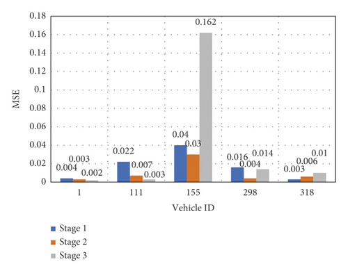
Figure 11 depicts MSE values in these stages for the five vehicles. As can be seen, the MSE values of the vehicles were low in Stage 2. This suggests that the developed NN-based LC model is capable of LC trajectory prediction in the LC stage. The errors of prediction, however, are relatively more significant and unstable in the first and third stages—for Vehicle 111 in Stage 1, Vehicle 155 in Stage 3, and Vehicle 298 in Stages 1 and 3. Mainly, Stages 1 and 3 proceed and follow LC implementation, respectively. In these stages, complex impact factors (i.e., the adjacent traffic states) could induce significant driving behavior uncertainty. Also, driving behavior heterogeneity adds to the uncertainty. Therefore, MSE somewhat fluctuates in the first and third stages, as shown in Figure 11. This suggests that a larger number of random impact factors exist in the adjustment stages before LC. As a result, the prediction has a greater difficulty.
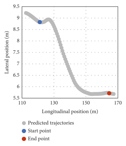
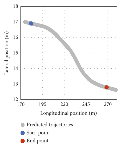
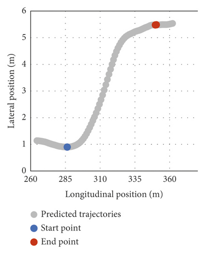
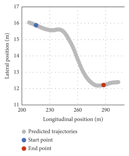
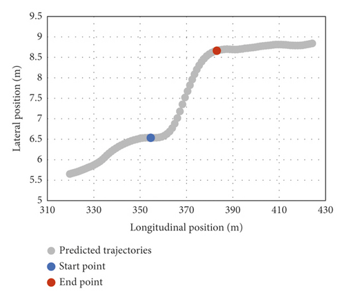
According to Figure 2, the beginning of LC behavior is considered to be a position in which the heading of the subject vehicle leaves the present lane direction, while the end of LC is a position in which the heading of the subject vehicle converges to the target lane direction. Thus, Figure 12 and Table 4 show the beginning/end prediction of the five vehicles’ testing data. Figure 12 illustrates some LC trajectories (in gray dots) of the testing data. The beginning points are shown in blue, while the endpoints are remarked in red. The beginning/end predictions are close to the observations. This implies that the beginning/endpoint predictions correspond to feasible LC behavior.
| Beginning point observation | Beginning point prediction | End point observation | End point prediction | |||||
|---|---|---|---|---|---|---|---|---|
| Vehicle ID | Lateral position (m) | Longitudinal position (m) | Lateral position (m) | Longitudinal position (m) | Lateral position (m) | Longitudinal position (m) | Lateral position (m) | Longitudinal position (m) |
| 1 | 8.8285 | 121.166 | 8.8231 | 121.114 | 5.70311 | 164.55 | 5.71682 | 164.559 |
| 111 | 16.9454 | 182.208 | 16.9071 | 182.093 | 12.8458 | 268.693 | 12.7861 | 268.629 |
| 155 | 0.88392 | 286.225 | 0.89471 | 286.33 | 5.44982 | 349.878 | 5.47811 | 349.71 |
| 298 | 15.8755 | 215.317 | 15.8763 | 215.227 | 12.2636 | 287.894 | 12.2182 | 287.848 |
| 318 | 6.51967 | 354.62 | 6.53608 | 354.638 | 8.64931 | 383.141 | 8.66336 | 383.134 |
6.3. LC Trajectory Predictive Performance
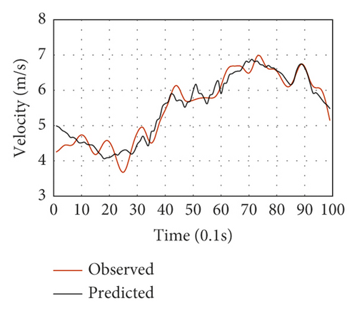
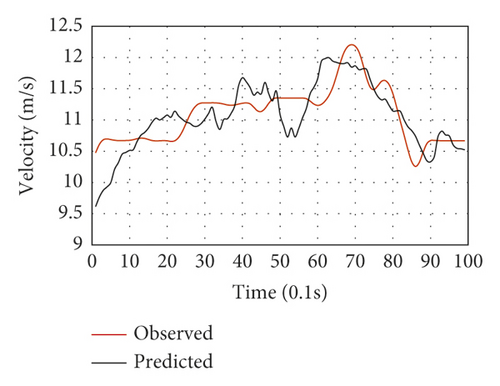
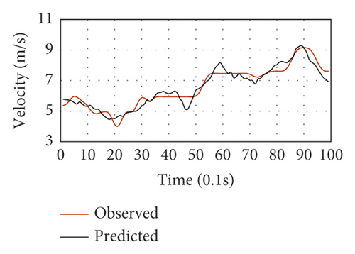
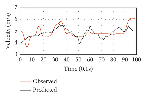
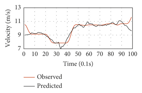
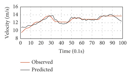
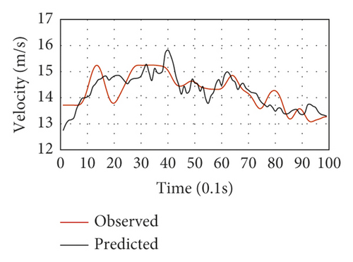
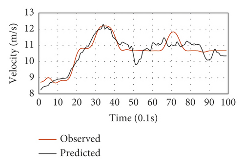
Figure 13 depicts the selected LC driving behavior results of the testing data. The cases with properly estimated LC trajectories and diverse speed variations were selected one by one to fulfill the proposed framework’s performance validation for various driving circumstances. Figures 13(a)–13(h) show the speed fluctuations of eight representative LC vehicles for LC maneuvers lasting ten seconds. The black lines represent the average speed prediction of each vehicle, while the red ones stand for the speed observations. These vehicles have no significantly large average speeds since the typical peak hour was utilized for validation. The introduced framework made proper trajectory estimates of all LC vehicles concerning the observed LC speed fluctuations. For the vehicles, the speed prediction MSE was utilized as a performance index throughout the LC process. Vehicles 1 and 298 had the lowest and highest MSE values, as shown in Figures 13(a) and 13(e), respectively. Concerning acceleration, the proposed model exhibited desirable performance in Figures 13(a), 13(c), and 13(f). Also, the LC trajectory estimates were found to be significantly close to the trajectory observations of the vehicles with large speed fluctuations for ten seconds in the LC maneuvers, as shown in Figures 13(b), 13(g), 13(d), and 13(h). For instance, complex impact factors (i.e., the adjacent traffic states) could induce significant driving behavior uncertainty before LC implementation. Also, driving behavior heterogeneity adds to the uncertainty. Consequently, there are large speed fluctuations in Figures 13(g) and 13(d).
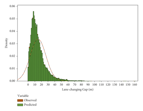
Additionally, for the characteristic validation of LC behavior, Figure 14 compares the NN-reproduced LC gap distributions to the real-life data. Also, Welch’s t-test was employed to evaluate the differences between the NN-reproduced distributions and the real-life data. Eventually, the p-value was found to be 0.998. A significantly higher p-value than 0.05 suggests a confidence level of 95% for assuming no significant difference between the prediction and real-life LC results. According to the results, the NN framework is capable of LC prediction and a decent indication of LC characteristics.
6.4. Comparison of SVR- and NN-Based LC Models
6.4.1. Supporting Vector Regression
Researchers have successfully developed and employed machine learning-based CF models in recent years, attempting to learn CF maneuvers through a massive amount of human driving CF data [44, 78]. Machine learning techniques may derive the CF behavior of drivers and capture the possible connections between different variables that could affect CF behavior. The present study adopted a machine learning framework for LC maneuver analysis and comparison to the introduced NN-based model. Concerning machine learning approaches, SVMs have been increasingly attractive in light of their high predictive performance. Several studies demonstrated SVMs to yield more satisfactory outcomes as compared to the results of statistical and other machine learning techniques [79, 80]. One can divide SVMs into classification SVMs and SVR machines. The former is employed for classification problems, while the latter is utilized for predicting continuous variables. SVR has proper generalizability and can deal with nonlinear problems. It has been successfully used for several real-life problems. SVR performs regularization error minimization and empirical risk minimization simultaneously with a proper penalty factor [81–83]. Consequently, the present work adopted SVR for LC trajectory prediction.
The SVR model was trained and tested using a personal computer with a 1.78 GHz CPU. To obtain optimal performance, SVR required a computational time of 4.0 s. The training and testing of SVR lasted for 540 s.
6.4.2. Comparison Results
As sufficient information on NN models was unavailable, we chose to adopt an NN-based LC model. In fact, NN success was a motivation of the work. Furthermore, CF approaches have recently been developed and applied based on machine learning. However, LC modeling has not been considered as frequently as CF modeling. To compare the proposed LC model, we adopted an SVR approach (machine learning) in order to analyze LC maneuvers. It was a challenging task to apply the SVR model with the same inputs as those of the NN. However, they both properly predicted trajectories with sufficient accuracy, capturing the longitudinal and lateral motions of the vehicles. Other models could be used for lane changing, but a review of data-driven LC researches indicates that NNs have been the most exciting instruments. Despite the development of some LCI and LCD-based NN approaches, a large number of questions remain yet to be answered, so that LC behavior could be understood. For example, long short-term memory (LSTM) could be a choice. According to the model inputs, which are spatial information in two dimensions (the lateral and longitudinal positions of the subject and four surrounding vehicles), we decided to use NN for LC prediction. As mentioned, NN success was a motivation of the authors. In fact, the use of the longitudinal and lateral vehicle positions as the NN inputs is the innovation of our work. Furthermore, LSTM takes more longer to train than NN, and LSTM is easy to overfit. Thus, the SVR and NN approaches can be said to have good performance. The NN-based and SVR-based LC models were compared. The same number of trajectories was employed for making comparisons. Also, the same set of data was utilized to train and test the SVR model in the form of an NN model. 15% of the data (i.e., sixty samples) were exploited in the testing phase, while 70% and 15% of the data were used for training and validation, respectively. Table 5 provides the MSE results of the two models. According to Table 5, the NN and SVR models yielded very close results.
| Model | MSE |
|---|---|
| NN | 0.023943 |
| SVR | 0.022643 |
Numerical tests were performed using the SVR model for the trajectory prediction of the sixty testing vehicles. MSE was utilized as an index of performance throughout the LC process. Figure 15 depicts the LC trajectory predictions of the testing vehicles (from the testing dataset).
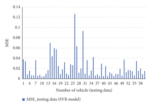
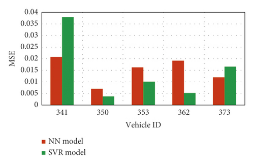
Figure 16 shows the MSE values of the SVR and NN models for five vehicles. Also, Figure 17 demonstrates the trajectory observations and predictions of the same vehicles. As can be seen, the two models’ trajectory predictions agree well with the observations and are capable of capturing lateral and longitudinal vehicle movements and SVR shows better performance than NN model. This, in turn, proves that the SVR and NN models have desirable performance. Furthermore, the results show that the SVR model is significantly similar to the NN model in trajectory prediction. A comparison of these models may demonstrate their ability to cope with overfitting.
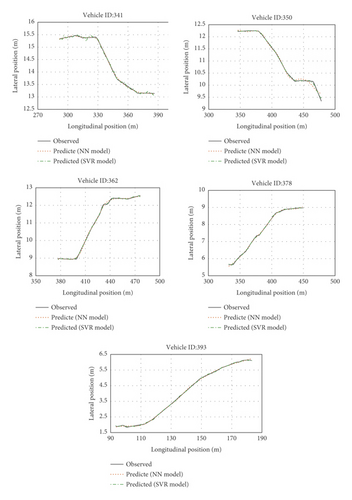
Additionally, the model’s predictive capability in reproducing macroscopic patterns can result from this study. The introduced models could make precise LC predictions of vehicles under small trajectory errors and satisfactory accuracy. In fact, NN and SVR models predict LC trajectories at time steps with the positions of both the subject and adjacent vehicles as the model input. After that, the effects of LC trajectory prediction can be seen in macroscopic patterns. For instance, the effect of LC trajectories on traffic flow at each time step predicted by proposed models can be determined and compared with the real data.
6.4.3. Comparison of Proposed Models with New Input Variables
The main innovative contribution is the parameters chosen for the model inputs. Finally, the proposed models were compared under various variables. To estimate LC behavior, it is required to select variables that could be measured using in-vehicle sensors. At the same time, it is important that multicollinearity is avoided by the traffic variables. For instance, since they have strong correlations, individual vehicle speeds and speed differences between different vehicles cannot be selected at the same time. Likewise, the vehicle type and gap are substantially intercorrelated and should not be simultaneously incorporated into the model. Eventually, a total of 11 variables were incorporated, as reported in Table 6.
| Variables | |
|---|---|
| Inputs | V(t) |
| d1(t) | |
| d2(t) | |
| d3(t) | |
| d4(t) | |
| V1(t) | |
| V2(t) | |
| V3(t) | |
| V4(t) | |
| X(t): lateral position of the subject vehicle | |
| Y(t): longitudinal position of the subject vehicle | |
| Outputs | X(t + ∆t): lateral position of the subject vehicle at next time step |
| Y(t + ∆t): longitudinal position of the subject vehicle at next time step | |
The MSE results of both the proposed models and the new ones with different variables are shown in Table 7. As can be seen, the proposed models yielded a lower MSE than the ones with new inputs, and there is significant difference between models with position and new inputs.
| NN and SVR models input | MSE (NN model) | MSE (SVR model) |
|---|---|---|
| Position variables | 0.023943 | 0.022643 |
| New variables | 2.42 | 1.26 |
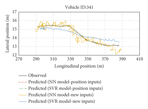
Table 8 shows the MSE values of the SVR and NN models for five vehicles under both the position inputs and new inputs. As can be seen, the two models’ trajectory predictions agree well with the observations and are capable of capturing lateral and longitudinal vehicle movements. This, in turn, proves that the SVR and NN models have desirable performance with position inputs. For instance, the observed and predicted trajectories of a vehicle under both the position inputs and new inputs are plotted in Figure 18. As can be seen, the trajectory predictions of the proposed models have greater consistency than the one with new inputs with the observed trajectories. Hence, the proposed models have higher performance than the new models. It can be said that information extraction from the lateral and longitudinal positions of the adjacent vehicles would yield much better outcomes than using new inputs for the prediction of the subject vehicle position by the NN and SVR models.
| Vehicle ID | NN model-position inputs | SVR model-position inputs | NN model-new inputs | SVR model-new inputs |
|---|---|---|---|---|
| 341 | 0.0207 | 0.0379 | 1.807 | 0.32 |
| 350 | 0.00699 | 0.0037 | 0.403 | 0.86 |
| 362 | 0.0162 | 0.01 | 0.372 | 2.91 |
| 378 | 0.0191 | 0.0052 | 1.011 | 1.532 |
| 393 | 0.0119 | 0.0165 | 0.185 | 2.468 |
7. Conclusion and Future Works
- (i)
The modeled results of the empirical data of vehicle trajectories revealed that the developed NN LC model could make accurate LC predictions of vehicles.
- (ii)
The experimental results suggested that the proposed technique could make accurate LC beginning/end estimates, demonstrating the beginning/end predictions corresponding to feasible LC behavior.
- (iii)
The performance evaluation of the NN model was performed through several trajectory data points of LC and adjacent vehicles, i.e., the following and leading vehicles, on the present and target lanes. The proposed model was found to yield proper LC trajectory estimates of all vehicles concerning LC speed observation fluctuations.
- (iv)
For the characteristic validation of LC behavior, the comparison of the NN-reproduced LC gap distributions to the real-life data was carried out. The characteristics of the LC gap distributions showed no statistically significant difference from real-life LC behavior.
- (v)
It was found that the SVR model was significantly similar to the NN model in LC trajectory prediction. A comparison of the two models demonstrated their capability of coping with overfitting.
- (vi)
The MSE results of both proposed models and the new ones with different variables have shown that the proposed models yielded a lower MSE than the ones with new inputs, and there is a significant difference between models with position and new inputs.
As future works, state-of-the-art models like game theory models would be considered for lane-changing modeling. Although the game theory approach has been used for modeling lane-changing decisions in the literature [1], lane-changing trajectory prediction can be tested with the game theory approach.
Also, the proposed model would be integrated in numerical simulations like AIMSUN. To integrate NN model in numerical simulations like AIMSUN, the output of NN model is used for calculating two local parameters (distance zones 1 and 2 [85]) that have the greatest influence on lane changing in AIMSUN. Then, these two local parameters are used in AIMSUN, and the average flows and speeds of all vehicles on the section are predicted by simulation model.
Conflicts of Interest
The authors declare that there are no conflicts of interest regarding the publication of this paper.
Open Research
Data Availability
The original NGSIM data is open to download at https://ops.fhwa.dot.gov/trafficanalysistools/ngsim.htm.


