
Optimization in the Ad Hoc On-Demand Distance Vector Routing Protocol
Abstract
The main challenge of the MANET network is the continuous management of information, each device, to ensure the correct direction of traffic. MANET consists of a peer-to-peer connection; the network is self-repairing and at the same time self-formed. The network can be used in the field of road safety, in sensors in the home, healthcare, robotics, etc. The aim of this work was to study the MANET network and its protocols and especially the AODV protocol, the choice of peer in the AODV protocol, and the subsequent improvement of this mechanism. The work deals with ETX metrics and its subsequent implementation in the AODV protocol. The work includes simulations of the AODV protocol and subsequently also simulations of the AODV-ETX protocol. The implementation of the proposed result simulation takes place in Network Simulator 3 tool. The work contains a comparison of the AODV and AODV-ETX protocols. The simulation results are shown in tables and plotted. The AODV-ETX has better properties compared to the AODV protocol, but with a larger number of nodes over 20, these properties approach the AODV protocol. The packet loss, packet delay, and permeability are considered for performance evaluations.
1. Introduction
1.1. MANET Network
An ad hoc network is one in which devices such as computers and cell phones communicate with each other using wireless devices [1–7]. In the MANET network, nodes (laptops, mobile phones, and other wireless devices) can move freely and completely randomly as the topology changes frequently [7–14]. Each node can act as a client and receive information or as a server that sends the provided data over the network. The structure of the MANET network is shown in Figure 1.

For network functionality, not all nodes need to be within range of all other nodes. If a station has radio reach to at least one of the elements in the network, it becomes a full member of this network [15–18]. The MANET works in the form of the enhanced output accuracy that helps to predict the form of the attack removal in such case of the denial of service attack etc. Thus, it helps to remove the attack or any other distortion in the entire network, thus helps to predict enhanced classification accuracy [19, 20]. Power Aware Routing Technique is used in the form of the enhanced accuracy and reduces the overhead in the entire function; thus, it provides the enhanced results in the overall results [21].
1.2. Routing Protocols in MANET
There are several types of routing protocols for wireless ad hoc networks. These routing protocols fall into two main groups: proactive and reactive. Routing protocols that use both proactive and reactive functions are called hybrid [22]. The distribution of routing protocols is shown in Figure 2.

1.2.1. AODV
AODV is an improvement of the DSDV algorithm. The protocol minimizes the amount of broadcast by creating routes on demand, while the protocol is DSDV, which maintains a list of all routes. In order for the node to find its way to the destination, it sends a route REQ packet using broadcast. Neighboring nodes broadcast a packet to another neighbor, the other until the packet reaches the node that has route information to the destination or until the route REQ packet reaches the destination. The node discards route REQ packets that it has already seen. These packets use a sequence number to ensure loop-free routes and to ensure that the node that responds to the request responds with only the most current information. This protocol uses only symmetric lines [23].
2. The Expected Transmission Count
The ETX (the expected transmission count) metric is one that seeks the path with the highest throughput in a multihop wireless network. The network with the smallest ETX has the highest throughput [24]. The ETX path metric is the estimated number of transmitted data needed to send a packet through this path to which the data forwarding is included. A packet that is not successfully received will be resent by the data sender.
2.1. Implementation of Link Probe Packets (LPPs) and ETX in AODV
- (i)
NeighborIpAddress. These are IP addresses of neighboring nodes
- (ii)
ReverseLppCount. It records the no. of LPP packets from neighboring node within the last 10 s
- (iii)
ForwardLppCount. It is obtained from the received LPP packets [26]. With these values for each neighboring node, the node can calculate the ETX metric for its neighbor at any time
In order for AODV to work with ETX metrics, ETX fields must be added to the protocol. In the AODV protocol, routing tables (RTs) are classified by destination according to the number of jumps. If the AODV finds multiple routing paths to the destination node, then the protocol selects the path that contains the least hops. With the modified AODV-ETX protocol, the path is classified on the basis of the ETX metric. The best path is the one that has the smallest ETX metric. If multiple paths are found that have the same metric, then the one that has the fewest jumps to the target node is selected [26].
ETX metrics are added by modifying RREQ and RREP packets. An additional field representing an ETX value is added to these packets. As soon as the source node Z sends an RREQ, the initial ETX value is set to zero. This is managed in the same way as the jump count field. As soon as the RREQ message is forwarded to the target node, the ETX metric is updated for each node based on Equation (3). The same procedure applies to the management of the RREP [26].
The ETX array is 32 bits in size. The calculated ETX value using Equation (1) and 104 is multiplied and rounded to the integer value. This will ensure that the ETX metrics work properly in Network Simulator 3 [26].
In the basic AODV protocol, nodes do not respond to any other RREQ message from a node from which they have already received the same message with the same ID.
However, this is different for AODV-ETX, and the receiving node from which the same message has already received the same message sends an RREP message if the ETX value from the received RREQ message is lower than the value recorded in the RT or even if the ETX value is the same, but the value of the number of jumps is lower [26].
3. Creating a MANET Network in NS-3
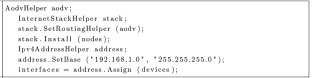
The freely distributable source code for AODV, which can be found on the NS-3 website, was used to create the MANET network and simulations. Header files and modules are added at the beginning of the code. These modules are used during the simulation run. A NodeContainer is then used to create and access nodes in the network, and nodes are created using the Create method. Nodes must have a defined grid layout. MobilityHelper and the SetPositionAllocator function are used to deploy nodes. Initial coordinates are represented by MinX, MinY, distance between nodes is represented by DeltaX, DeltaY, no. of nodes placed in the network is represented by GridWidth, and node layout method (RowFirst or ColumnFirst) is represented by LayoutType. In this network, the nodes are arranged in a row, the distance between them is 50 meters. 20 nodes are used, the mobility of which is constant, and so they do not move. To ensure that the nodes can communicate with each other via the wireless channel, the WifiMacHelper, YansWifiPhyHelper, and YansWifiChannelHelper helpers are used. Then, using the Install method, the parameters such as physical and line addresses to individual nodes are assigned. Finally, the creation of pcap files is turned on, which we will view in Wireshark. The files contain the communication of all nodes in the created network. The AODV protocol is used as a routing protocol in the simulation. In the code, it looks like this:
The address space for the created nodes is created thanks to Ipv4AddressHelper. To create traffic in the created network, it is necessary to create an application that generates packets. V4PingHelper is used in our simulation. The ApplicationContainer object installs applications on the source node. It also determines when the application should start working and when it should end. The simulation is set to 60 seconds, and we also set the end of the ping. During the simulation, node 4 is moved away from the other nodes so that we can capture the RRER message in the communication between the nodes. Node removal is accomplished by the following code snippet:
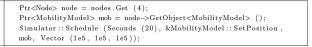
where in 20 seconds, node 4 moves out of the other nodes. The simulation is started with Simulator :: Run and shuts down with Simulator:: Stop when the tasks are completed. We will use the waf tool to run the simulation. # ./waf - run scratch/Manet Test.
3.1. AODV Protocol Simulation
We can also start the simulation with a graphical representation. We will use the command to start such a simulation # ./waf - run scratch/Manet Test – vis. As soon as the command is entered into the terminal, a statement will appear in the terminal stating that we have run a simulation with 8 nodes, which are 50 meters apart, and this simulation will last 60 seconds. Each node has a range of 60 meters. An extract from the terminal is in Figure 3.

As soon as the simulation starts, we will also see a graphical representation of our network Figure 4 in which we can see the nodes we have created. In this part of the simulation, all nodes are in a row, where in time 20 seconds, node number 4 moves out of our topology and thus node 0, which communicates with node 7, loses connection. In this simulation, a packet loss of 66% occurs. The first 20 packets sent pass, and as soon as node 4 ceases to exist in the topology, the other packets cannot be delivered to the destination node. The topology in this simulation is constant, meaning that the nodes do not move.

After 60 seconds, the simulation is over and the ns-3.30.1 folder stores pcap files that can be opened in Wireshark. After opening Wireshark, we can see the communication of each node. After opening the pcap files of individual nodes, I set the filter to the AODV protocol. At time 0 seconds, node 0 requested the RREQ message Figure 5 to find out the destination to the destination of node 7 with the destination IP address 192.168.1.8. He then received an RREP response from a nearby node, which asked for his neighbor's RREQ message to travel to node 7 and then made an entry to node 0 utilising the return path method.

The communication then continued to the node 6, which received the RREQ message within 1,189 seconds, with the destination IP address. node 7, the source address of node 0, the hops 5, and the seq. number 4 from node 5. Node 0 sent up to 4 RREQ messages until a connection was established with node 7. Node 6 had node 7 recorded in the RT, so it sent him an RREP message at time 1,192 to inform node 7 that node 0 wanted to connect to it. Likewise, node 6 sends an A-flag RREP to neighboring node 5 that it knows the path to node 7. Node 5 must then send an RREP acknowledgment message to node 7. Node 0 at time 1,252 receives an RREP message from node 1 with seq. number 0 and hops to node 7.
This completes the process of finding out the route and in the selected simulation at 8 nodes in a row, where the first node communicates with the last one took 1.252 seconds. Communication between nodes 0 and 7 continued for up to 20 seconds. At 20 seconds, node number 4 disconnected from the topology and a space was created between nodes 3 and 5, through which communication could no longer take place. As soon as node 4 was not part of the topology, node 5 sent an RRER message with the following content:
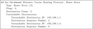
This terminates the communication between nodes 0 and 7, because in this case, the simulation does not have points that are moving and so the communication could not continue. All other messages from node 0 have been dropped. For comparison, additional simulations were performed, shown in Table 1. All simulations start from time 0 s, after the first RREQ message is sent from the source side to the last node in the topology.
| Number of nodes | First RREQ (s) | RREP (s) |
|---|---|---|
| Three | Zero | 0.252 |
| Eight | Zero | 1.241 |
| Fifteen | Zero | 2.027 |
| Twenty | Zero | 2.130 |
| Thirty | Zero | 2.231 |
3.1.1. Simulation with RandomRectanglePositionAllocator Layout
In this type of simulation, the nodes in our network are created in random positions. We achieve this by using the ObjectFactory class. All described simulations are based on a communication scenario where node 0 (the first node of the created topology) communicates with the last node of the topology. For a 15-node network, these are nodes 0 and 14. Simulation parameters include simulation area (100 m × 100 m), number of nodes (15), simulation duration (60 seconds), distance of nodes from each other (random), and range of knots (60 meters). After entering the command into the terminal to start the simulation, the nodes are arranged randomly and immediately after starting the simulation, and node 0 starts the route discovery process shown in Figure 6. Once they find the route to node 14, they begin to communicate with each other. The entire communication takes place through the neighboring node 9, as in Figure 7.


Each node maintains its own RT, which contains the destination IP address, the path through which the neighboring node will get there, the interface, the route marker, the route expiration time, and the number of hops from the destination. From the simulation, parts from the three RTs of nodes 0, 9, and 14 are selected through which communication takes place. In the Wireshark program in Figure 8, it can be seen that node number 9 was the first to respond to the call of node 0 and sent an RREP, with the number of hops 1 and so node 0 established a connection through this node. Node 10, which is a neighboring node and also has a number of hops 1, sent an RREP message 0.001 s later.

3.1.2. Simulation with RandomRectanglePositionAllocator and RandomWaypointMobilityModel
The most common situation we can encounter at MANET is node mobility. Each subscriber node in the network moves, and the routing must change along with it. The RandomWaypointMobilityModel will help us design such a simulation. Initial simulation parameters include simulation area (100 m × 100 m), number of nodes (5), simulation duration (60 seconds), distance of nodes from each other (random), and range of knots (60 meters). In this simulation, we will then use the visualization tool NetAnim. The tool is part of NS-3, and to use it, you need to add the following lines to the source code:
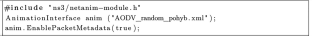
At the end of the simulation, we can notice that with 5 nodes and a space size of 100 meters per 100 meters, we have a packet loss of 10%. You can see the simulation display in the NetAnim graphical environment in Figure 9.

The results of other simulations are shown in Table 2. The results of the simulations show that adding nodes to the network increases our loss and packet delay. As the nodes move, the line between the source and the destination is often interrupted, so the discovery process must occur again, thus increasing the line delay.
| Number of nodes | Packet loss (%) | RTT (round-trip time) avg (ms) |
|---|---|---|
| Ten | 5 | 2277 |
| Fifteen | 7 | 327 |
| Twenty-five | 11 | 767 |
| Thirty-five | 37 | 1092 |
| Forty | 42 | 1816 |
3.2. Comparison of AODV and AODV-ETX Protocols
Two simulation scenarios were used to simulate the ADOV and AODV-ETX protocols.
3.2.1. Simulation with Constant Arrangement of Nodes
The same source codes used by the ConstantPositionMobilityModel were used in the simulation. In the model, node 0 client communicates with node 19 server. Initial simulation parameters include protocol used for communication (ns3:: UdpSocketFactory), number of nodes in the simulation (20), simulation duration (20 seconds), distance of knots from each other (50 meters), and range of knots (100 meters). Both protocols chose a route with the number of jumps 7. Selections of these routes are shown in the figures below. The AODV protocol has chosen the route shown in Figure 10, and the AODV-ETX protocol has chosen the route shown in Figure 11.


From all tests, we obtained the following results shown in Table 3. The AODV (A) and AODV-ETX (B) protocols do not differ when the nodes are constantly arranged. The nodes have similar paths, the same number of jumps, and also the same loss, so the results of the simulation are almost identical. We will also use the RandomWalk2dMobilityModel to test the differences between the two protocols, where the results will better represent the difference between the protocols.
| Baud rate (kbps) | Protocol | Number of hops | Throughput (kbps) | Packet loss (%) | Average packet delay (ms) |
|---|---|---|---|---|---|
| 100 | B | Seven | 95.992 | 6.98 | 16.251 |
| 100 | A | Seven | 95.991 | 6.98 | 16.331 |
| 120 | B | Seven | 115.094 | 7.01 | 14.685 |
| 120 | A | Seven | 115.095 | 7.01 | 14.723 |
| 140 | B | Seven | 133.952 | 7.22 | 13.570 |
| 140 | A | Seven | 133.951 | 7.21 | 13.580 |
| 160 | B | Seven | 153.053 | 7.22 | 12.694 |
| 160 | A | Seven | 153.053 | 7.22 | 12.712 |
3.2.2. Simulation Using RandomWalk2dMobilityModel
This type of simulation consists of different node movements within our created network. There are always two static nodes in the simulation, namely, node 0 client and the last node in the simulation server. The parameters were used in the simulation include protocol used for communication (ns3:: UdpSocketFactory), number of nodes in the simulation (different), bit rate (300 kbps), simulation duration (20 seconds), distance of knots from each other (50 meters), range of knots (80 meters), and node movement speed (1.5 m/s). At the beginning of each simulation, the nodes are laid out in a grid, according to the rule 5 nodes per line. When simulating 13 nodes, the network looks like this in Figure 12.

After starting the simulation, node 12 starts communicating with node 0 within 1 second. As soon as the simulation is started, all nodes except nodes 0 and 12 start moving at a constant speed. Communication and node layout after 13 seconds from the start of the simulation looks like Figure 13.

The simulations were performed for the AODV protocol and the AODV-ETX protocol with the same parameters as well as with the same installation of the Ubutnu Linux system and at the same time with the NS-3 simulation environment version 3.30.1. The results of the simulation when changing the variable number of nodes are described in Table 4.
| Number of hops | Protocol | Throughput (kbps) | Packet loss (%) | Average packet delay (ms) |
|---|---|---|---|---|
| Ten | B | 214.35 | 38.155 | 150.546 |
| Ten | A | 134.34 | 58.072 | 148.090 |
| Thirteen | B | 227.20 | 22.971 | 36.554 |
| Thirteen | A | 189.96 | 35.581 | 33.286 |
| Sixteen | B | 157.72 | 74.781 | 38.283 |
| Sixteen | A | 134.92 | 79.437 | 47.202 |
| Eighteen | B | 201.85 | 23.132 | 20.181 |
| Eighteen | A | 198.37 | 30.361 | 9.991 |
| Twenty-two | B | 171.26 | 30.762 | 32.144 |
| Twenty-two | A | 176.73 | 30.521 | 17.211 |
The results show that the AODV-ETX protocol has better properties when setting up communication in an environment where nodes move. We can notice that when increasing the number of nodes above 20, the AODV-ETX protocol no longer has as good results as with smaller numbers of nodes in the network. The results shown in Table 4 were plotted in graphs (Figures 14–16), respectively.


4. Conclusion
The aim of this work was to study the MANET network and its protocols and especially the AODV protocol, the choice of peers in the AODV protocol, and the subsequent improvement of this mechanism. This work describes the creation of the MANET network in NS-3, and there are added lines from the code that is used in all simulations. The work contains commands for starting the simulation, statements from the terminal, and graphical representations of these simulations. At the end of the work, simulations of the AODV protocol and the AODV-ETX protocol are created. The selection of peers in the AODV protocol relies only on the number of hops, while in the AODV-ETX protocol, the ETX metric is applied to ensure the route with the best throughput. The simulation results show that the proposed protocol has better efficiency compared to the AODV protocol, but with a larger number of nodes over 20, these properties approach the AODV protocol. In future enhancement, this work can be improved with an optimization algorithm and with an efficient path routing protocol. It is employed to track reliable paths.
Conflicts of Interest
There is no conflict of interest.
Open Research
Data Availability
The datasets used and/or analyzed during the current study are available from the corresponding author on reasonable request.