Rotating Machinery Fault Identification via Adaptive Convolutional Neural Network
Abstract
Rotating machinery plays an important role in transportation, petrochemical industry, industrial production, national defence equipment, and other fields. With the development of artificial intelligence, the equipment condition monitoring especially needs an intelligent fault identification method to solve the problem of high false alarm rate under complex working conditions. At present, intelligent recognition models mostly increase the complexity of the network to achieve the purpose of high recognition rate. This method often needs better hardware support and increases the operation time. Therefore, this paper proposes an adaptive convolutional neural network (ACNN) by combining ensemble learning and simple convolutional neural network (CNN). ACNN model consists of input layer, subnetwork unit, fusion unit, and output layer. The input of the model is one-dimensional (1D) vibration signal sample, and the subnetwork unit consists of several simple CNNs, and the fusion unit weights the output of the subnetwork units through the weight matrix. ACNN recognizes the self-adaptive of weight factors through the fusion unit. The adaptive performance and robustness of ACNN for sample recognition under variable working conditions are verified by gear and bearing experiments.
1. Introduction
As a key component of mechanical transmission system, rotating machineries have been widely used in the transmission system of automobiles [1], ships [2], wind turbine [3], machine tools, etc. However, in the actual industrial scene, they are easy to be broken down due to the harsh service environment and variable speed and load [4, 5]. So, it is vulnerable to catastrophic accidents if health state of equipment is not considered in a timely manner. Therefore, the research on intelligent and efficient recognition model is of great significance to ensure the healthy operation of equipment [6–8].
At present, the common monitoring technology can be divided into three groups: index-based trend forecast methods, spectrum signal-based analysis methods [9], and data-driven deep learning (DL) methods [10, 11]. The former two rely heavily on expert experience and require more labour input. In the past decade years, benefiting from the rapid development of computer systems and intelligent sensing technologies, deep learning methods have been attached to too much attention. As an end-to-end fault diagnosis technology, deep learning aims to build a learning model and mine the inherent complex mapping between feature space and fault types by learning massive labeled data, to predict and judge diagnosis of unknown samples. Existing favourable deep learning methods include deep belief network (DBN), Auto-Encoder (AE) [12], and convolutional neural network (CNN) that present significant advantages in solving varieties of classification problems. Wang proposes a deep interpolation neural network (DICN) [13], which improves the fault recognition rate of neural network under time-varying conditions. Eren et al. [14] used compact 1D-CNN to extract recognition features from the original fault data, and the classification time is less than 1 msec, which is very suitable for the fact monitoring and diagnosis of mechanical equipment. Zhang et al. [15] proposed a deep convolutional neural network with wide first-layer kernels (WDCNN) which used the wide kernels in the first convolutional layer for extracting features and suppressing high-frequency noise. Liu et al. [16] proposed a multiscale kernel-based residual CNN (MK-ResCNN) which overcomes the problem that the gradient of deep network disappears, and used multiscale nuclear energy to extract fault features more accurately. Du et al. [17] proposed a convolution sparse learning model for deconvolution of complex modulation of transmission path, and successfully detecting the transient fault impulses of gearbox vibration signal. Huang et al. [18] used minimax concave penalty function to construct an objective function and constraint the sparsity coefficients. As a result, the repetitive transient’s information is effectively extracted. Li et al. [19] proposed a power spectral entropy based variational mode decomposition method and introduced it into deep neural networks, and achieve a promising fault recognition rate. Li et al. [20] proposed a named WaveletKernelNet framework where the first layer of a standard CNN is replaced with continuous wavelet transform, achieving an interpretable feature map with clear physical meaning. Sun et al. [21] combined sparse auto-encoder SAE with DNN and presented a SAE-based CNN to learn more differentiated features of unlabeled data, and experimentally verified its effectiveness. Guo et al. [22] established a named hierarchical learning rate adaptive deep convolution neural network where the two-dimensional (2D) CNN hierarchical framework with an adaptive learning rate is adopted to recognize bearing fault categories and sizes. Cheng et al. [23] proposed a hybrid time-frequency analysis method, which was successfully used for railway bearing fault identification, which could effectively recover fault information from raw signals contaminated by strong noise and other interferences.
With the research and development of intelligent recognition methods, the scale of the model is becoming larger and larger in order to pursue high recognition rate, which obviously does not correspond to a good direction of fault diagnosis. The large scale of intelligent recognition model needs better hardware support and increases the recognition operation time, which is obviously unfavourable to the industrial application of intelligent recognition methods. Therefore, this paper proposes an adaptive convolutional neural network (ACNN) by combining ensemble learning and simple convolutional neural network (CNN). ACNN model consists of input layer, subnetwork unit, fusion unit, and output layer. The input of the model is one-dimensional (1D) vibration signal sample, and the subnetwork unit consists of several simple CNNs, and the fusion unit weights the output of the subnetwork units by the weight matrix. The weight matrix can adjust the proportion of each subnetwork output, increase the influence of identifying the correct subnetwork unit output, and weaken the influence of identifying the wrong subnetwork output. ACNN realizes the integrated learning of the model by adaptively adjusting the simple CNN as the output of the basic classifier, which can improve the recognition rate of the model without significantly increasing the network parameters. The adaptive performance and robustness of ACNN for sample recognition under variable working conditions are verified by gear and bearing experiments.
- (1)
ACNN is proposed by combining ensemble learning with simple 1D-CNN, which can accurately identify rotating machinery faults under unknown working conditions. It provides a new idea and method for intelligent fault diagnosis
- (2)
ACNN replaces the combination strategy in traditional bagging ensemble learning with optimized weight parameters. The combination strategy is optimized by continuously optimizing the weight parameters
- (3)
The proposed ACNN is generalizable, and it can also be applied to other machine learning algorithms. Besides, it can be also found that the proposed ACNN not only has a good identification performance for multiple load conditions but also shows a strong ability to unknown information representation for samples under variational working conditions, including speed, load, and oil
The rest of this paper is organized as follows. Section 2 presents theoretical background. In Section 3, the architecture of ACNN is proposed and the training strategy of model is introduced. In Section 4, compared with other network architectures, the fault diagnosis results of the ACNN are discussed on the gearbox dataset and bearing dataset, and the validity of the model is verified. Section 5 concludes this paper.
2. Theoretical Background
The model proposed in this paper is based on one-dimensional (1D) CNN theory and reference learning. The 1D-CNN is essentially a multilayer perceptron, which adopts the method of local receptive fields and shared weights. On the one hand, this method reduces the number of weights and makes the network easy to optimize; on the other hand, it reduces the risk of overfitting. The 1D-CNN is generally composed of input layer, 1D convolution layer, activation function, pooling layer, and full connection layer, as shown in Figure 1.
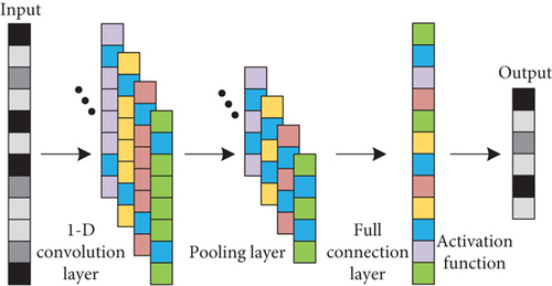
The high-dimensional spatial feature map obtained after the input data that is subjected to the convolution operation will be inputted to the pooling layer for subsampled processing. The most commonly used pooling operation is the max-pooling operation. The max-pooling operation will divide the feature map into several nonoverlapping regions according to the relevant parameters and step size of the pooling region, and then extract the maximum value in each region as the representative value of this region, and discard other values of this region. The maximum values of different regions are sequentially combined into a new feature map as the output of the pooling layer.
3. Adaptive Convolutional Neural Network
3.1. Motivation
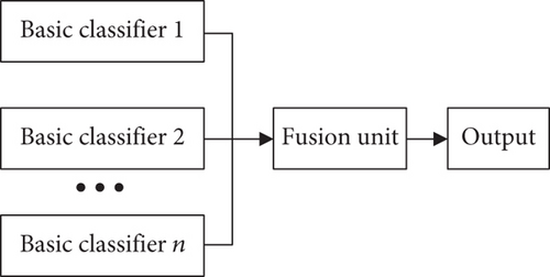
The ensemble learning refers to a machine learning method that integrates multiple basic classifiers with certain criteria or strategies in order to obtain a strong learner to achieve the target task. For a complex problem, multiple experts have given different opinions and solutions. If you can discuss these different opinions and methods, and get a comprehensive opinion and solution, it is often more comprehensive and better than any one of them. Ensemble learning is based on this idea to complete the learning task. Its concept can be summarized as follows: For a specific target task, use sample data to train to obtain a few base learners with certain training criteria and strategies and then use appropriate fusion criteria or algorithm, which integrates multiple basic classifiers to obtain a strong classifier with excellent performance to complete the target task. Figure 2 shows the general structure of ensemble learning. The traditional bagging is an algorithm that optimizes the output of weak learners by combining strategies. The bagging algorithm not only improves its accuracy and stability but also avoids overfitting by reducing the variance of the results. The voting average method is a common combination strategy. However, the traditional combination strategy cannot be updated. We use the network weight parameters to replace the traditional combination strategy, and continuously adjust the output weight of each weak classifier through the network parameter update iteration. Combining the idea of bagging algorithm with CNN, an ACNN framework is proposed.
3.2. ACNN Architecture
The ACNN model is mainly composed of the following four parts: input layer, subnetwork unit, fusion unit, and output layer. The input layer is used to receive the time-domain signal and input it to the subnetwork unit, which architecture is shown in Figure 3. The subnetwork unit is composed of 1D-CNN fault identification subnetworks. The number of subnetworks is consistent with the number of working conditions (speeds or loads) of samples in the training dataset. Each subnetwork has the same structure and corresponds to different working conditions, respectively. ACNN can accurately extract the fault-sensitive information of rotating machinery under variable working conditions and accurately identify the fault type. The fusion unit stores the weight matrix obtained through supervised training, which is used to assign different weights to the output results of the subnetwork, then performs fusion learning and outputs the final recognition results.
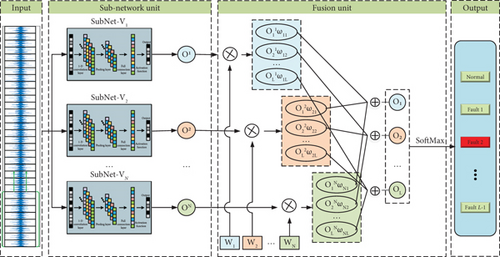
The processing process of the input data by the subnetwork unit is shown in Figure 3. During fault identification, a fault sample to be identified is input into the ACNN; the input layer receives the sample and inputs it into the subnetwork unit. Each subnetwork receives the sample and is activated, and uses the stored fault type information and sample feature distribution information to learn and identify the sample.
Among them, the subnetwork corresponding to the input sample speed condition will output the original fault identification results with high accuracy, and other subnetworks will show inconsistent responses. Therefore, the construction of subnetwork unit realizes the transformation of fault identification problem under multiple working conditions into fault identification problem under single working condition, that is, for each known working condition fault sample to be identified, there is a subnetwork identification module with high identification accuracy corresponding to its working condition. After the subnetwork unit completes the processing of the input data and obtains the original recognition results O1, O2, …, ON, it inputs the original recognition results O1, O2, …, ON to the fusion output layer for the next step. When the multi subnetwork unit completes the processing of input data and obtains the original identification results O1, O2, …, ON, we input the result to the fusion output layer for weighted information fusion learning, as shown fusion unit in Figure 3. The original identification results O1, O2, …, ON are output by different CNN fault identification subnetworks. The identification subnetworks consistent with the working conditions of the input samples will output high-accuracy fault identification results, while other identification subnetworks will output low-accuracy fault identification results. In other words, after the fusion output layer performing weighted fusion learning on the input original identification results O1, O2, …, ON, high-accuracy fault identification results occupy a large proportion in the final identification results, and the results with low accuracy are suppressed, so that the accuracy of the final identification results is guaranteed.
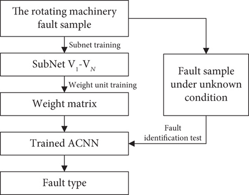
3.3. ACNN Training
- (1)
Extracting the time-domain signals of fault vibration at different conditions in the actual industrial scene, construct the fault sample set under all conditions
- (2)
Divide the fault sample set into sample sets under different conditions, and then train the subnetworks and weight matrix of ACNN model
- (3)
Put the fault sample under a certain condition in the same scene into the trained ACNN network model to obtain the fault type corresponding to this sample
4. Experimental Verification and Analysis
The performance of ACNN is verified on gear dataset and bearing dataset. The gear dataset [24] came from Chongqing University, and the bearing dataset came from Case Western Reserve University (CWRU) [25].
4.1. Case I: Gear Dataset
- (1)
Test platform and dataset description
The schematic diagram of the structure of the gear test bench is shown in Figure 5. It consists of five parts: the drive motor, the two-stage spur gear reducer, the speed sensor, the magnetic powder brake, and the control cabinet. The speed of the drive motor and the load of the magnetic powder brake are controlled by the control cabinet, which enable the gearbox to run stably under various speeds and loads. The transmission ratio of the two-stage spur gear reducer is 3.59, the gear ratio of the first transmission stage is 23/39, and the gear ratio of the second transmission stage is 25/53. The motor is a DC motor of YVFF-112M-4, with rated power of 4 kw, rated voltage of 380 V, and maximum speed of 1200 rpm. The magnetic particle brake model is CZ10, rated voltage is 380 V, rated current is 1.2A, and can provide controllable stable torque load for the experimental system within 0 to 500 N.
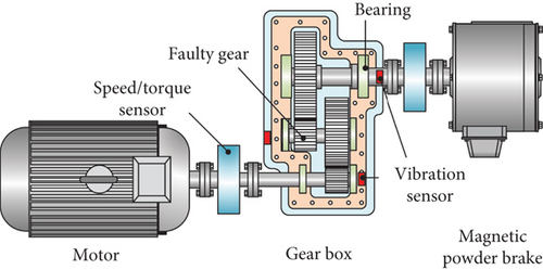
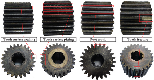
The structural parameters of the gearbox are shown in Table 1. The fault gear is the intermediate transmission gear with 25 teeth. The gear faults include tooth surface spalling, root crack, tooth surface pitting, and tooth fracture, which are shown in Figure 6. The vibration sensor is set in the vertical direction of three transmission shafts. The training and test data are obtained from the vibration signal of the middle drive shaft position sensor.
| Number of high-speed gear teeth | Number of low-speed gear teeth | Transmission ratio | Center distance |
|---|---|---|---|
| 23 | 25 | 1.696 | 93 mm |
| 39 | 53 | 2.12 | 117 mm |
The gear fault and vibration acquisition settings are shown in Table 2.
| Fault type | Fault size (mm) | Input speed (rpm) | Sampling frequency (Hz) | Sampling time (s) |
|---|---|---|---|---|
| Healthy | None | 700, 750, 800, 850,900, 950, 1000, 1050, 1100 | 20480 | 15 |
| Tooth surface spalling | 60 × 3 × 0.5 | |||
| Root crack | 60 × 3 | |||
| Tooth surface pitting | 2 mm | |||
| Broken tooth | 30% tooth width (18 mm) |
- (2)
Classification comparison and analysis
| Datasets | Train sets | Test sets | Number of training/testing samples |
|---|---|---|---|
| A | 600, 900 rpm | 500 to 1100 rpm | 10000/65000 |
| B | 800, 1100 rpm | 10000/65000 | |
| C | 500, 700, 900 rpm | 15000/65000 | |
| D | 550, 750 950 rpm | 15000/65000 |
In order to verify the advantage of ACNN, CNN [14], residual networks (ResNet) [26], wide first-layer kernels (WDCNN) [15], and multiscale kernel-based ResCNN (MK-ResCNN) [16] are used as comparison networks. The comparison models and ACNN are built based on Python 3.7 and Pytorch 1.7.1. The main configurations of the computer are as follows: CPU-i9-9900k, RAM-128GB, GPU-RTX 2080Ti. The five methods (ACNN, DCNN, ResNet, WDCNN, and MK-ResCNN) are trained and tested by the datasets in Table 3; the classification results are shown in Figure 7.
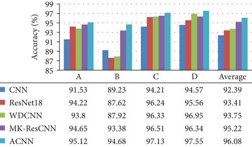
There is no cross sample between the training set and the test set. This verification method is also called fixed dataset verification. It can better verify the recognition ability of the recognition model to unknown working condition samples and improve the robustness. The recognition rates of CNN, ResNet, WDCNN, MK-ResCNN, and ACNN are 91.53%, 94.22%, 93.8%, 94.65%, and 95.12% on dataset A, respectively. The recognition accuracy of ACNN model is higher than that of the other four comparison models. The sample recognition rate of ACNN model is also higher than that of other models on datasets B, C, and D. The average recognition rate of ACNN is 3.69%, 2.67%, 2.33%, and 0.86% higher than that of CNN, ResNet, WDCNN, and MK-ResCNN, respectively. Although the recognition rate of MK-ResCNN model is close that of ACNN model, the network parameter number of MK-ResCNN is more than three times that of ACNN model, and its training time is longer. The experimental results show that ACNN has high recognition rate and strong robustness. The recognition accuracy of datasets C and D samples is higher than that of datasets A and B, because the training set of datasets C and D contains more speed samples, which is also reasonable. The confusion matrix of the identification result on dataset D is shown in Figure 8.
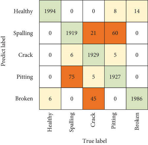
It can be found that the recognition accuracy of healthy samples is the highest by the confusion matrix of the recognition results. There are 75 samples of tooth surface spalling fault incorrectly classified as tooth surface pitting corrosion. The number of tooth surface pitting fault samples incorrectly identified as tooth surface spalling is 60. This shows that the fault characteristics of tooth surface spalling and tooth surface pitting are similar. The number of tooth root crack fault samples incorrectly identified as tooth surface spalling and tooth fracture is 21 and 45, respectively. The parameters and calculation time of the comparison model on dataset A are shown in Table 4. It can be found that the parameters of ACNN network are less than those of the comparison model, and the training and testing time are the least.
| Models | Training time (s) | Testing time (s) | Model parameter quantity |
|---|---|---|---|
| CNN | 0.501 | 0.304 | 211672 |
| ResNet18 | 1.015 | 0.156 | 661508 |
| WDCNN | 0.241 | 0.162 | 99270 |
| MK-ResNet | 3.395 | 1.261 | 835274 |
| ACNN | 0.116 | 0.128 | 54076 |
4.2. CWRU Bearing Data
- (1)
Test platform and data description
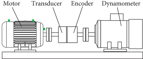
The experimental data are collected from the accelerometer of the motor-driven mechanical system (Figure 9) at a sampling frequency of 12 kHz. There are four kinds of bearing faults, that are normal, inner ring fault, ball fault, and outer ring fault. The fault dimensions of the three fault kinds are divided into 0.007 inch, 0.014 inch, and 0.021 inch. Therefore, there are 10 kinds of bearing states that need to be classified. The failure frequency of bearing fault types (inner ring fault, outer ring fault, and ball fault) is different, so we use this data to verify the performance of ACNN.
- (2)
Classification comparison and analysis
| Datasets | Train datasets | Test datasets | Number of training/testing samples |
|---|---|---|---|
| A | 0, 1 hp | 2, 3 hp | 8000/8000 |
| B | 0, 2 hp | 1, 3 hp | 8000/8000 |
| C | 0, 3 hp | 1, 2 hp | 8000/8000 |
| D | 1, 2 hp | 0, 3 hp | 8000/8000 |
| E | 1, 3 hp | 0, 2 hp | 8000/8000 |
| F | 2, 3 hp | 0, 1 hp | 8000/8000 |
| G | 1,2, 3 hp | 0 hp | 12000/4000 |
| H | 0, 2, 3 hp | 1 hp | 12000/4000 |
| I | 0, 1, 3 hp | 2 hp | 12000/4000 |
| J | 0, 1, 2 hp | 3 hp | 12000/4000 |
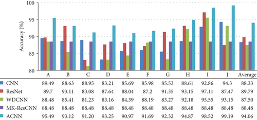
In order to verify the advantage of ACNN, CNN [14], residual networks (ResNet) [26], wide first-layer kernels (WDCNN) [15], and multiscale kernel-based ResCNN (MK-ResCNN) [16] are used as comparison networks. The five methods (ACNN, DCNN, ResNet, WDCNN, and MK-ResCNN) are trained and tested by the datasets in Table 5; the classification results are shown in Figure 10. The recognition accuracy of ACNN is 95.49%, which is 6%, 5.79%, 7.01%, and 13.24% higher than CNN, ResNet, WDCNN, and MK-ResCNN on bearing dataset A, respectively. The recognition accuracy of ACNN is 93.12%, which is 4.49%, 0.01%, 7.11%, and 10.84% higher than CNN, ResNet, WDCNN, and MK-ResCNN on bearing dataset B, respectively. The average recognition rates of ACNN, CNN, ResNet, WDCNN, and MK-ResCNN models on bearing datasets are 94.06%, 88.33%, 8.79%, 87.50%, and 86.06%, respectively. The average accuracy of ACNN is more than 4.28% higher than that of other comparison models, which proves that ACNN has strong recognition performance and adaptability to samples under variable load conditions. In order to explore the identification details of samples by ACNN model, the confusion matrix of the output results of dataset A is shown, which is shown in Figure 11.
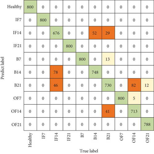
In the confusion matrix, it can be found that all health status samples are correctly classified, and the number of 0.014 inch inner ring fault samples incorrectly identified as ball faults is 124. The number of ball fault samples incorrectly identified as outer ring fault is 81. This shows that there are similarities between inner ring fault characteristics and ball fault characteristics. The parameters and calculation time of the comparison model on dataset A are shown in Table 6. It can be found that the parameters of ACNN network are less than those of the comparison model, and the training and testing time are the least.
| Models | Training time (s) | Testing time (s) | Model parameter quantity |
|---|---|---|---|
| CNN | 0.401 | 0.043 | 211672 |
| ResNet18 | 0.812 | 0.022 | 661508 |
| WDCNN | 0.193 | 0.023 | 99270 |
| MK-ResNet | 2.716 | 0.180 | 835274 |
| ACNN | 0.093 | 0.018 | 54076 |
5. Conclusions
This paper proposes an adaptive convolutional neural network by combining ensemble learning and simple convolutional neural network. ACNN model consists of input layer, subnetwork unit, fusion unit, and output layer. The input of the model is one-dimensional (1D) vibration signal sample, and the subnetwork unit consists of several simple CNNs, and the fusion unit weights the output of the subnetwork units by the weight matrix. In gear and bearing experiments, the performance and robustness of ACNN model are verified by comparing with CNN, ResNet, WDCNN, and MK-ResCNN models.
Conflicts of Interest
The authors declare that they have no conflicts of interest.
Acknowledgments
This work was supported by Chongqing Natural Science Foundation (cstc2019jscx-msxm X0360, cstc2019jcyj-msxmX0346), National Natural Science Foundation of China (under Grant No. 51805051), and the Central University Basic Research Fund (2020CDJGFCD 002).
Open Research
Data Availability
Data available on request.


