With the advent of the information age, the need for information technology construction is beginning to be realized when working in corporate financial management. The application of ERP systems to financial management has become a major trend in the development of modern society. This can help companies collect financial information in real time and analyze and process the obtained information. This paper first gives the significance and models of the ERP financial management system. Then, a financial risk prediction model based on a deep learning model is designed. The method proposes an improved temporal convolutional network-long and short-term memory network (TCN_LSTM) structure and introduces an optimization algorithm to optimize the parameters of the deep learning model. Finally, several benchmark models and evaluation methods are used for comparative study. The experimental results show that the deep learning risk prediction model has significant superiority in prediction accuracy and stability. The proposed model can help enterprises organize their limited resources, realize the scientific allocation of enterprise resources, and create more benefits for enterprises.

1. Introduction

Financial management is an essential part of an enterprise related to the enterprise’s overall development. It is very important to do an excellent job in the financial management of the enterprise to obtain long-term and stable growth [1, 2]. In the information age, the use of information technology tools should be strengthened in enterprise management. The Enterprise Resource Planning (ERP) system [3], an essential method of financial management, is a product of the development and changes in the information age. The ERP system provides reliable support for the rational application of information technology in enterprises.

ERP system combines an enterprise’s production and financial management based on providing information technology for the enterprise [4]. It enables the finance department to obtain accurate business data promptly, which is conducive to the rational use of resources, thereby improving efficiency and optimizing the effectiveness of capital use. This effectively improves the management level of enterprise finance and promotes the rational use of funds. However, the effect of such multidepartmental collaboration is difficult for most enterprises to achieve. In the traditional enterprise financial management model, each department is relatively independent of the other and not closely enough connected. They cannot realize real-time information sharing and effective communication, which easily leads to untimely access to information and poor decision-making. Therefore, the level and efficiency of enterprise financial management are not high and eventually may cause great losses to the company [5]. Enterprises should speed up familiarizing themselves with the use and application of ERP systems and change to a systematic and integrated direction. The use of ERP can improve the overall management efficiency of the enterprise and reduce the risk of decision-making and error rate of the enterprise.

Enterprise financial management is an important part of enterprise management. It can improve financial management by establishing and improving a financial management system, increasing control over enterprise financial risks, reducing economic decision-making errors, and improving financial management. Enterprise financial management has a very important significance for the development of enterprises. The ERP system is an important part of the enterprise financial management system [6]. The ERP system provides data sharing functions and multiangle and multilevel observation of the development of the enterprise to achieve timely detection and problem-solving. This can reduce the enterprise’s risk in financial control and continuously improve the financial management system of the enterprise to promote its overall development [7].

Financial risk forecasting for financial firms is an important part of the ERP financial management system. Early financial risk forecasting models were mainly based on traditional statistical models. However, these models are mainly linear and have strict assumptions, which cannot portray the nonlinear relationship of financial risks. This makes the accuracy of financial risk prediction low and cannot meet the practical requirements of an early financial warning. With the rapid development of computer technology and artificial intelligence, methods such as support vector machine (SVM) [8] and random forest (RF) [9] have been applied to the field of economic forecasting. These nonlinear forecasting methods have significant advantages in dealing with complex nonlinear problems [10]. As one of the most popular methods, SVM can find the optimal decision hyperplane by minimizing the structural risk and has good generalization ability. In [11], a risk prediction model with kernel fuzzy twin SVM was designed for early warning of systemic financial risks. However, SVM and NN are shallow machine learning methods with the problems of invalid feature representation and the inability to learn complex high-dimensional data effectively.

The advantage of deep learning is that it extracts complex and effective features by learning step by step through multiple networks [12], which has higher prediction accuracy and generalization ability. Lv et al. [13] used deep neural networks for stock trading prediction, and the experimental results showed that DNNs have good prediction potential for financial time series. In a study on predicting the daily closing price of the Dow Jones Industrial Index, Ouyang et al. [14] found that LSTM neural networks are effective in capturing the variability of financial time series. Fewer studies have applied deep learning to financial risk prediction. Furthermore, the choice of parameters can have an important impact on the prediction effectiveness of the model [15]. The main optimization methods regarding the model parameters include cross-validation, grid search, and intelligent optimization algorithms. Bataineh and Kaur [16] utilized the CSA algorithm to optimize the setting of the weights of the feedforward neural network.

The aforementioned studies have generally used single-objective optimization methods, but enterprise financial risk forecasting is affected by various factors, and it is necessary to consider not only the forecasting accuracy but also the model stability. Xue et al. [17] introduced the NSGA-III multiobjective algorithm to forecast the electric load. The results show that the forecasting performance of the optimized model after NSGA-III is significantly better than that of the single-objective model. The representative multiobjective optimization algorithms mainly include PAES, SPEA2, and NSGA-II [18]. Among them, MOPSO is a multiobjective optimization algorithm based on Pareto domination and external archiving mechanism, which has the advantages of good convergence characteristics and low time complexity [19, 20]. In a comparative study with other multiobjective optimization algorithms. MOPSO significantly outperforms methods such as NSGA-II, PAES, and mi-croDE [21].

In order to improve the performance of risk prediction in ERP financial management systems, this work proposes a TCN_LSTM prediction model with improved MOPSO to achieve high-accuracy prediction of enterprise financial risk based on the research mentioned above.

The innovations and contributions of this study are as follows:

(1)
An ERP enterprise financial management model is designed.
(2)
TCN_LSTM is constructed by the multiconvolution kernel parallel network for multisource time feature extraction.
(3)
TCN_LSTM introduces dilation convolution to achieve multiscale feature extraction and expand the perceptual field to improve the processing efficiency of memory units. Residual linkage is introduced to the TCN_LSTM model to enhance the gradient propagation capability.
(4)
The MOPSO optimization algorithm is enhanced to improve the financial risk prediction performance of the TCN_LSTM network.

This study consists of four main parts: the first part is the introduction, the second part is the methodology, the third part is the result analysis and discussion, and the fourth part is the conclusion.

2. Methodology

2.1. The Significance of ERP for Enterprise Financial Management

Figure 1 gives the significance of ERP for corporate financial management, which is reflected in six aspects.

(i)
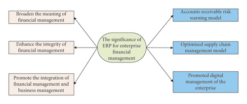
Broadening the connotation of financial management: under the traditional business model, enterprises mainly focus on material procurement, capital management, equipment management, revenue management, and other aspects of financial management. In patent technology, human resources, customer management, sales management, accounts receivable management, cost management, and other aspects lack effective control. In intangible assets, accounting and management are more difficult to obtain the desired management effect. By applying the ERP system, we use a modern system to analyze and evaluate all enterprise assets. Moreover, in the role of supply chain management, risk assessment, financial accounting, production management, human resource management, and other modules, ERP systems effectively expand the scope of corporate financial management.
(ii)
Enhancing the integrity of financial management: in addition to being able to prepare financial statements, the ERP system can also integrate and manage various financial data. Various departments can use the ERP system to effectively transfer financial information, which is conducive to the sharing of financial data, thereby preventing information delays. This gives the enterprise financial management work smoothly to provide data reference so that financial management is more standardized and professional.
(iii)
Promoting the integration of financial management and business management: in the traditional financial management model, financial information and business information are in a separate state, which is not conducive to the orderly integration of business and financial work of enterprises. By using the ERP system, financial and business information can be integrated to form a more complete and intuitive data map. Finance staff and managers can use the data chart to combine business and finance. They can have a comprehensive understanding of the overall business situation, which is conducive to the integration of business and financial information.
(iv)
Accounts receivable risk warning model: the use of an ERP system can enhance the management of enterprise funds; for example, the system can integrate and code the various resources required in the production process. Collecting the relevant codes can help the enterprise know the material inventory, price, and other information. The system can update the data when materials are used and deployed to other departments. In the ERP system, a risk warning module can be set up. For example, if the receivable period exceeds the agreed recovery period in accounts receivable management, the system automatically issues an early warning message. This facilitates the relevant departments to deal with it in time to prevent the risk of bad debts and doubtful debts and ensure the enterprise’s interests.
(v)
Optimizing supply chain management model: in implementing supply chain management, enterprises are required to combine internal and external resources and customer needs and use each link in the supply chain as an enterprise ally. In supply chain management, it is necessary to combine customer needs and provide professional products or services for customers. By adjusting the internal and external processes of the production enterprise, the product circulation time is shortened, and the logistics speed is accelerated. This allows customers’ individual needs to be met in a short time and creates more benefits for the company.
(vi)
Promoting digital management of the enterprise: we establish an enterprise-wide, system-wide, and module-wide data monitoring platform using the ERP system. The enterprise is dynamically supervised, thus realizing the digital management of the enterprise. By conducting regular business analysis meetings, we provide accurate financial information to business operators and managers with the help of an ERP system.

Details are in the caption following the image — Open in figure viewer PowerPoint

2.2. Module Analysis of ERP in Enterprise Financial Management

Figure 2 illustrates the ERP enterprise financial management system model. The model is divided into the accounting, accounts receivable, information, fixed assets, and financial management modules.

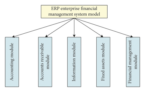
Accounting Module. The value of the accounting module is understood through the functional analysis of the ERP system. This can facilitate the technical accounting of the enterprise and truly show the business process and results. Through the survey and analysis, accounting involves the general ledger, payroll accounting, and cost, among others. The general ledger module can process the bookkeeping vouchers and complete the input and registration. The payroll module automatically accounts for and allocates employees’ salaries and completes the accrual of funds in conjunction with related expenses. In contrast, the cost module calculates and completes production planning based on the structure of products produced by the enterprise, production process, and procurement information in operation and production. Using the standard cost averaging method can control the production cost.

Accounts Receivable Module. The accounts receivable module includes invoice management, account management, and customer management. It transforms relevant events into specific vouchers to be imported into the general ledger by combining them with customer orders, invoice processing operations, and so on. In calculating accounts receivable, financial risk predicting needs to be fully integrated with the purchasing module and inventory module from multiple perspectives of invoice management, voucher management, and supplier management. This can form a complete management pattern and improve enterprise management.

Information Module. The information module allows you to control cash flow and complete petty cash accounting and analysis, including cash and checks. The information module can be connected with the accounts receivable and accounts payable modules to automatically form vouchers posted to the general ledger system.

Fixed Assets Module. The fixed assets module enables fixed asset changes, asset accruals, and asset accounting, which provides an effective way of asset management through this module. The fixed assets module includes fixed assets cards and detailed accounts, which automatically form vouchers.

Financial Management Module. This module can provide a data basis for the development of accounting. Financial management solutions are derived by combining previous financial situations in financial planning. Query work is provided in financial analysis, and data differentiation is completed through user customization. As the focus of account management, financial decision-making can help enterprises make feasible financial decisions. Taking various management countermeasures to connect the company’s production process ensures that the company reduces inventory and improves efficiency.

Risk forecasting is an important part of the ERP financial management system. This study gives the financial risk forecasting model design in Section 2.3.

2.3. Financial Risk Forecasting Model Design

2.3.1. TCN-LSTM

Several factors influence financial risk prediction. This study combines the improved TCN and LSTM to construct the TCN_LSTM risk prediction model. The model can improve the accuracy and computational efficiency of forecasting. Its network structure is shown in Figure 3. The number of hidden layers is not limited to the two layers in the figure, and the arrows pass the hidden layer states from left to right by moment.

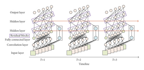
First, an improved TCN model is used to effectively combine multidimensional financial data for risk prediction while maintaining the causal convolution property. Secondly, the dilation convolution is introduced into the standard LSTM to realize the extraction of higher-order features and filtering of useless information from financial data using its efficient feature extraction. This can improve the efficiency of LSTM hidden layer memory unit processing. Finally, the overall network structure of the prediction model is optimized by incorporating residual links. It directly transmits features across layers, simplifies the overall data feature learning process, and enhances the gradient propagation capability. The specific process is as follows:

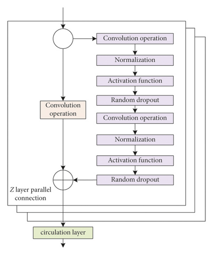
(1) Initialize the TCN Model Structure and Parameters. In financial risk forecasting, the input is usually multidimensional financial data, including profitability, operating capacity, fixed cash flow capacity, and debt service capacity. The standard TCN model has only a one-dimensional convolution kernel, so it can only handle one-dimensional input data. In this study, multiple one-dimensional expansion convolutions are operated in parallel in multiple dimensions to construct a set of multiple parallel networks of separable one-dimensional convolution kernels. The parallel network is used to extract the implicit feature information in each dimension and perform feature fusion, which fully preserves the correlation between financial data in different dimensions and can greatly improve the efficiency of model operations.

A schematic diagram of the one-layer multiple one-dimensional dilation convolution process is shown in Figure 4. The input data X is a matrix of w × t consisting of t kinds of data with a total time span of w. After the action of the convolution filter F_n of size d × 1 and the dilation factor D of 2 in the convolution layer, the output N is t feature maps, where the t th feature map is subjected to the dilation convolution operation by the input X_t and the convolution filter F_t, which is calculated by the following formula:

(1)

For the one-layer multidimensional convolution operation demonstrated in Figure 4, the perceptual field size is calculated by the following formula; that is, the perceptual field of the convolution kernel of this layer is 7∗7 = 49:

(2)

For multilayer multidimensional convolutional nets in TCN_LSTM, the recursive formula for calculating the sensory field size is as follows:

(3)

where S_x denotes the x th layer step size. Z_t denotes the nth layer convolution kernel size. The convolution kernel size is calculated as follows:

(4)

where U denotes the padding value in the network model. After such multiple convolution operations on the input data, the abstract features contained in the financial data are effectively extracted. Moreover, the links between features can still be maintained for various data classes. The output matrix with the same dimension as the input dimension is obtained through the full convolution layer in TCN after a multilayer convolution operation.

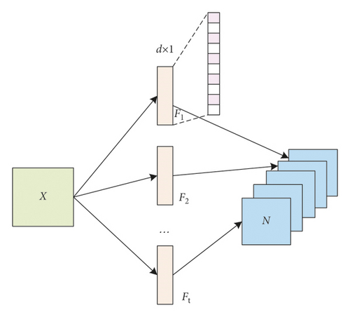
The improved TCN model retains the original dilated and causal convolution features while covering the full range of dimensional data inputs from the original unidimensional financial data. This fully ensures that it can handle financial data effectively and speed up the training speed of the network model with a better sense of real-time feedback.

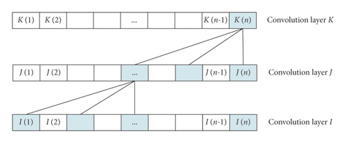
(2) Initialize the LSTM Model Structure and Parameters. The more standard LSTM model in dealing with long-term memory, due to the long history, multispecies data optimization storage capacity, lack of prediction accuracy degradation, and prediction feedback delay problem. In this work, we extract the amount of dependent information contained in the current moment n by adding the dilation convolution operation before the recurrent layer of the LSTM network. For the same size of input data, the larger the sensory field contained in the network, the fewer the number of network layers required to extract all the data. This significantly simplifies the network structure and optimizes the network processing speed and prediction accuracy.

The dilation convolution operation is illustrated in Figure 5. The convolution kernel size is set to 3, and the dilation rate is 1. The effective information contained in the convolution layer K at time n is a higher-order feature extracted from the information contained in the convolution layer I from time 1 to time n. This feature can filter the useless information in the long-time data very efficiently while preserving the correlation between the original multidimensional information. This can reduce the amount of data for subsequent processing and improve the overall processing efficiency.

After the convolution layer operation processes the financial data, the higher-order features of the multidimensional financial sequences are passed through the full connection layer into the recurrent layer to obtain the output results. The predicted results are then compared with the historical financial real-world data. The errors calculated in the output layer are used for gradient backpropagation to update the configuration of each parameter in the recurrent layer. The financial risk model with the smallest loss function value is selected when the maximum number of iterations is reached.

(3) Introduce Residual Links for the Overall Model. Considering that the improved TCN_LSTM runoff prediction model needs to learn multidimensional data over a long period, the network convolution layers still have a very large number. Moreover, after multilayer convolution and compression operations, the dependent information still has some differences and losses compared with the original information. Therefore, the residual linking method is introduced in the network model to enable the network to transfer the underlying dependency information across layers. This can maximize the output layer to fuse the higher-order features with the detailed underlying features and improve the prediction accuracy.

A residual block consists of a direct mapping part and a residual part, which is expressed as

(5)

where i_t represents the dependency information embedded in the t th convolution layer. C represents the dilation convolution operation, that is, the direct mapping part. F is the residual mapping operation performed between different layers. The convolution layers in this model consist of multiple convolutional kernels in parallel to perform deep-level feature extraction. In contrast, multiple generic residual blocks are designed and combined to perform multidimensional feature extraction from source data. Two layers of dilated causal convolution and activation function ReLU are included in each residual block layer, and the weights are applied to normalize the convolution kernels. In addition, dropout is added after each dilated causal convolution for regularization to mitigate the occurrence of overfitting of source features. The structure diagram is shown in Figure 6. For the Z-layer parallel residual block, the source data are input into the residual function of each layer. An additional layer of dilation convolution is utilized to ensure that the same shaped tensor is obtained to resolve the different input and output widths.

(4) Model Optimization. In this study, an improved MOPSO algorithm is designed for parameter optimization of the depth model. It is particularly important how the inertia weights balance the global searchability and the local searchability. Usually, the inertia weights are set in a linear decreasing strategy in the optimization process. However, suppose the linear decreasing strategy is adopted to update the inertia weights in the optimization process. The global search ability will be stronger if the values are larger in the first iteration. This is easy to jump out of the local optimum and help find the global optimum. In the later iterations, the inertia weights become smaller, and the global search ability becomes weaker, whereas the local search ability becomes stronger. At this time, the convergence speed becomes faster, so it is not conducive to jumping out of the local optimum, and thus the phenomenon of premature maturity occurs. This study adopts the strategy of updating inertia weights by nonlinear function and resetting unfavorable particles by the Gaussian distribution model to solve the drawbacks of using a linear decreasing strategy. In the weight update, the inertia weight of the improved algorithm gradually increases in the first half iterations and decreases in the second half iterations. In the standard PSO algorithm, the update of each dimensional value of each particle velocity takes the same inertia weight. However, the amount of change of each dimensional value of the particle is not the same. The improved MOPSO algorithm adopts different inertia weights to update some particle velocity dimensions. The inertia weights are calculated as follows:

(6)

where ω_xd is the inertia weight of particle x in the d th dimension. ω_min, ω_max are the lower and upper limits of the inertia weight, respectively. L is the maximum number of iterations. δ is the fluctuation coefficient of the inertia weight. R1, R2 are the random numbers obeying uniform distribution in the interval [0, 1] and [−1, 1], respectively.

Updating the inertia weights using only line and nonlinear functions is not effective in increasing the diversity of the population. When a particle flies in the opposite direction, the particle may fall into a local optimum. A uniformly distributed random number is assigned to the particle flying in an unfavorable direction within the definition of particle position. Each random value has the same probability and is not targeted. In the iterative particle position update process, the particle positions are selectively reset using random values generated by the Gaussian distribution model for particles flying in an unfavorable direction considering the problems mentioned above. This makes the particle population more diverse and reduces the possibility of the algorithm falling into a local optimum. In order to make the assigned values more specific, the mean and variance of the Gaussian distribution model are determined using the current particle position, the individual historical optimal position, and the optimal global position. The position is updated as follows:

(7)

where

(8)

2.3.2. Risk Projections

The optimal model is obtained by pretraining using historical financial data. The test samples are input into the model for calculation. Finally, the risk prediction data are obtained and compared with the actual test set to obtain the model prediction results.

Figure 7 presents the flow of the prediction model based on deep learning. The overall model is initialized with the model structure, hyperparameters, and preprocessing of the multisource data to screen out erroneous data, such as 0 values, null values, and other cases. The multisource data are then constructed as a multidimensional matrix and used as data input. Null convolution is performed on the data in the convolution layer to extract high-dimensional features. This step can effectively reduce the number of high-dimensional network layer weight coefficients and significantly reduce the overall model spatiotemporal complexity. The convolved high-dimensional features are fed into the loop layer for computation via the full connection layer.

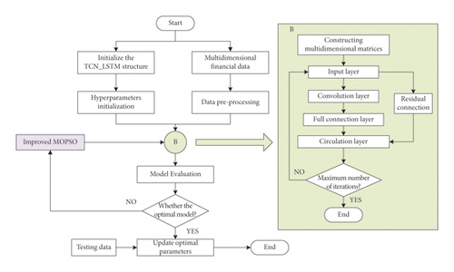
In contrast, the residual link spanning layer is used to transfer the unprocessed data from the bottom layer into the loop layer, which is used to prevent data loss and distortion caused by multiple cycles of the complex network layer. The loss values of the model for each iteration are then recorded. The optimal model for each iteration round is recorded. When the maximum number of iterations is reached, the optimal results are compared, and the model with the smaller loss value is output. This optimal model is taken as the final result and tested using the test set to obtain the TCN_LSTM model prediction results.

3. Result Analysis and Discussion

3.1. Financial Risk Forecasting Model Evaluation Indicators

This study analyzes the classification accuracy of the financial risk early warning model using the traditional classification correct rate, and the prediction accuracy of the financial risk early warning model is evaluated using the evaluation indexes for unbalanced samples. The evaluation indexes and calculation formulae are given in Table 1.

1. Description of evaluation index.

Index: calculation formula	Meaning
TPR = (TP/TP + FP)	Positive sample prediction correct rate
TNR = (TN/TN + FN)	Negative sample prediction correct rate
TR = (TP + TN/TP + FP + TN + FN)	Overall accuracy rate
	Geometry average correct rate. If G is larger, the model predicts both types of samples with higher accuracy. Conversely, the smaller the accuracy of the model, the lower the correct rate will be.
F = ((2 × (TN/(TN + FN)) × (TN/(TN + FP)))/((TN/TN + FN) + (TN/TN + FP)))	Few classes of samples metric. If F is larger, the model has superior predictive performance for the financial risk class sample and vice versa for a few classes of sample measures

3.2. Selection of Feature Indicators

Because there is no accepted standard for the characteristic indicators used in the financial risk prediction model, this study draws on relevant studies to select the characteristic indicators. A risk warning system containing financial and nonfinancial indicators was initially obtained. Finally, 13 groups of indicators, such as development capacity, profitability, and solvency, were selected as the input features of the financial risk prediction model, as shown in Table 2. In this study, the above indicators are selected to build a feature index set.

2. Description of model characteristics indicators.

Classification	Variable type	Number of variables
Financial indicators	Development capacity	8
	Solvency	10
	Profitability	10
	Operating capacity	10
	Fixed cash flow capacity	10
	Revenue quality	2
	Innovation capability	2
	Risk tolerance	3

Nonfinancial indicators	Macroeconomic indicators	2
	Market information	2
	Corporate governance	4
	Management incentives	3
	Shareholding structure	5

The PCA method is used to reduce the dimensionality of the indicators. The KMO and Bartlett’s spherical tests are performed before PCA to determine whether each indicator is suitable for principal component analysis. The test results show that the KMO value of financial risk forecast indicators is 0.65, and the p value of Bartlett spherical is significant, indicating a relatively obvious correlation between the indicators, which is suitable for PCA analysis. In addition, the cumulative contribution of the principal components corresponding to the top 33 eigenvalues exceeds 91% according to the Kaiser–Harris criterion, parallel analysis, and Cattell’s gravel test. Therefore, the top 33 principal components will finally be selected as training data for input into the deep learning model in this study.

3.3. Prediction Performance Comparison

3.3.1. Comparison of Prediction Accuracy

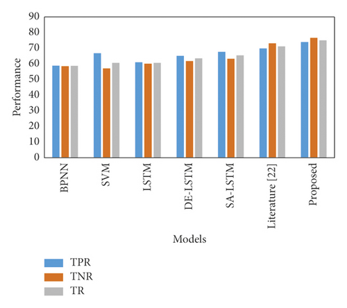
There are six types of comparison models, including BP neural network (BPNN), SVM, long short-term memory network (LSTM), differential evolutionary algorithm-LSTM (DE-LSTM), simulated annealing-LSTM (SA-LSTM), and NSGA–II–DNN model in [22].

The comparison of the model’s prediction accuracy in this study and the comparison model is given in Figure 8. The combined results show that the model constructed in this study has the best prediction accuracy. Its evaluation indexes TPR, TNR, and TR are 73.89%, 76.57%, and 75.05%, respectively, higher than the other six prediction models, which indicates that the model has better performance in enterprise financial risk forecasting. In addition, the better prediction performance of the models in [22] and in this study indicates that the multiobjective optimization algorithm outperforms the single-objective approach in terms of prediction effectiveness.

The above experimental results analyzed the differences of the models only in terms of the numerical magnitude of the prediction accuracy and lacked mathematical and statistical significance. Therefore, in order to strengthen the scientific and objective nature of the obtained results, a paired-samples t-test was used for significance testing to determine whether there were significant differences in the prediction performance of different models. The specific experimental results are shown in Table 3.

3. Paired samples t-test for prediction accuracy of each model.

Models	Proposed
Models	TPR	TNR	TR
Literature [22]	5.027 ^∗∗∗	3.437 ^∗∗	7.303 ^∗∗∗
SA-LSTM	12.442 ^∗∗∗	8.315 ^∗∗∗	20.497 ^∗∗∗
DE-LSTM	13.147 ^∗∗∗	8.748 ^∗∗∗	17.494 ^∗∗∗
LSTM	9.269 ^∗∗∗	8.911 ^∗∗∗	10.626 ^∗∗∗
SVM	6.283 ^∗∗∗	33.799 ^∗∗∗	18.88 ^∗∗∗
BPNN	23.978 ^∗∗∗	24.443 ^∗∗∗	32.264 ^∗∗∗

Note: ^∗ indicates p < 0.1, ^∗∗ indicates p < 0.05, ^∗∗∗ indicates p < 0.01.

The results in Table 3 show that the null hypothesis is rejected at the 1% significance level for the t-test on each indicator for the proposed model and the proposed model except for the paired sample t-test on TNR for the proposed model and [22] which is significant at the 5% level. It indicates that the proposed model is significantly different from the other models on TPR, TNR, and TR, and its financial risk prediction is better.

3.3.2. Comparison of Prediction Stability

Because paired sampling according to the 1 : 1 ratio will have some impact on the randomness of the samples, this study tests the robustness of the model by varying the ratio between positive and negative samples. Firstly, the ratios between financial risk samples and normal financial samples are set to five, 1 : 2, 1 : 3, 1 : 4, 1 : 5, and 1 : 6, respectively. Then, the changes in prediction accuracy of the four types of models under these five ratios are analyzed. Thus, the prediction stability of the proposed model is judged. Given that the samples under the five ratios no longer belong to balanced samples, it is necessary to introduce a metric specifically for unbalanced samples to evaluate the model’s prediction performance. The results of the model experiments are shown in Figure 9.

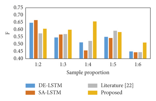
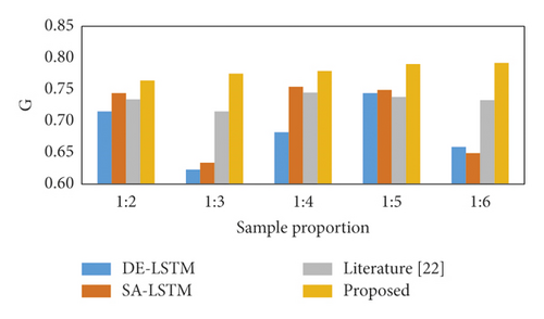
The proposed model has a higher G value (0.7800) than the other models for different positive and negative sample ratios. The proposed model performs poorly in terms of F value, but its F mean (0.5910) is higher than the other models with the smallest standard deviation. This indicates that the literature [22], DE-DNN, and SA-DNN models are worse than the proposed models for financial risk and normal financial samples. Graphically, the prediction accuracy of the proposed models G and F are relatively smoother and less volatile in trend, indicating that the prediction results are stable for the two types of samples with different financial sample ratios.

4. Conclusion

By analyzing and discussing the significance of the ERP financial management system, we design a model of an ERP-based enterprise financial management system. A deep learning financial risk prediction model is proposed to analyze and process financial data in ERP. In this study, prediction fully considers the complexity of financial risk prediction, combines multiobjective optimization algorithm and deep learning technology to construct an ERP enterprise financial risk hybrid prediction model, and compares it with six other benchmark models. The results show that, first, the model in this study has a much better prediction capability in terms of prediction accuracy. Compared with other methods, its prediction accuracy is statistically significant. Second, in terms of prediction robustness, the model in this study can effectively control the fluctuation of prediction accuracy and improve prediction stability. Compared with [22], SA_LSTM, and DE_LSTM, the prediction accuracy G value (mean) is improved by 4.7%, 7.40%, and 9.54%, respectively. The future research direction is to refer to multiple MOPSO-optimized deep learning models for the risk prediction of ERP financial management systems to improve system performance.

Conflicts of Interest

The author declares that there are no conflicts of interest.

Acknowledgments

This study was supported by the Hunan Institute of Traffic Engineering.

Open Research

Data Availability

The labeled dataset used to support the findings of this study is available from the corresponding author upon request.

References

1 Yuniningsih Y., Pertiwi T. K., and Purwanto E., Fundamental factor of financial management in determining company values, Management Science Letters. (2019) 9, no. 2, 205–216, https://doi.org/10.5267/j.msl.2018.12.002, 2-s2.0-85058536731.
10.5267/j.msl.2018.12.002
Google Scholar
2 Prihartono M R D. and Asandimitra N., Analysis factors influencing financial management behaviour[J], International Journal of Academic Research in Business and Social Sciences. (2018) 8, no. 8, 308–326, https://doi.org/10.6007/ijarbss/v8-i8/4471.
10.6007/IJARBSS/v8-i8/4471
Google Scholar
3 Febrianto T. and Soediantono D., Enterprise resource planning (ERP) and implementation suggestion to the defense industry: a literature review[J], Journal of Industrial Engineering & Management Research. (2022) 3, no. 3, 1–16.
Google Scholar
4 Bamufleh D., Almalki M. A., Almohammadi R., and Alharbi E., User acceptance of enterprise resource planning (ERP) systems in higher education institutions, International Journal of Enterprise Information Systems. (2021) 17, no. 1, 144–163, https://doi.org/10.4018/ijeis.20210101.oa1.
10.4018/IJEIS.20210101.oa1
Google Scholar
5 Atmadja A. T., Saputra K. A. K., Tama G. M., and Paranoan S., Influence of human resources, financial attitudes, and coordination on cooperative financial management[J], The Journal of Asian Finance, Economics, and Business. (2021) 8, no. 2, 563–570, https://doi.org/10.13106/jafeb.2021.vol8.no2.0563.
10.13106/jafeb.2021.vol8.no2.0563
Web of Science® Google Scholar
6 Alhalboosi F. H. A., Mawlood S. J., and Al-halboosi I. A. M., Role of ERP systems in improving human resources management processes[J], Review of International Geographical Education Online. (2021) 11, no. 4, 1667–1681, https://doi.org/10.48047/rigeo.11.04.155.
10.48047/rigeo.11.04.155
Google Scholar
7 Alzahrani A., Mahmud I., Thurasamy R., Alfarraj O., and Alwadain A, End users’ resistance behaviour paradigm in pre-deployment stage of ERP systems: evidence from Bangladeshi manufacturing industry, Business Process Management Journal. (2021) 27, no. 5, 1496–1521, https://doi.org/10.1108/bpmj-08-2019-0350.
10.1108/BPMJ-08-2019-0350
Web of Science® Google Scholar
8 Rostami O. and Kaveh M., Optimal feature selection for SAR image classification using biogeography-based optimization (BBO), artificial bee colony (ABC) and support vector machine (SVM): a combined approach of optimization and machine learning, Computational Geosciences. (2021) 25, no. 3, 911–930, https://doi.org/10.1007/s10596-020-10030-1.
10.1007/s10596-020-10030-1
Web of Science® Google Scholar
9 AlThuwaynee O. F., Kim S. W., Najemaden M. A., Aydda A., Balogun A. L., Fayyadh M. M., and Park H. J, Demystifying uncertainty in PM10 susceptibility mapping using variable drop-off in extreme-gradient boosting (XGB) and random forest (RF) algorithms, Environmental Science and Pollution Research. (2021) 28, no. 32, 43544–43566, https://doi.org/10.1007/s11356-021-13255-4.
10.1007/s11356-021-13255-4
CAS PubMed Web of Science® Google Scholar
10 Saadat M. and Bayat M., Prediction of the unconfined compressive strength of stabilised soil by adaptive neuro fuzzy inference system (ANFIS) and non-linear regression (NLR), Geomechanics and Geoengineering. (2022) 17, no. 1, 80–91, https://doi.org/10.1080/17486025.2019.1699668.
10.1080/17486025.2019.1699668
Google Scholar
11 Huang X. and Guo F., A kernel fuzzy twin SVM model for early warning systems of extreme financial risks, International Journal of Finance & Economics. (2021) 26, no. 1, 1459–1468, https://doi.org/10.1002/ijfe.1858.
10.1002/ijfe.1858
Web of Science® Google Scholar
12 Venugopalan J., Tong L., Hassanzadeh H. R., and Wang M. D., Multimodal deep learning models for early detection of Alzheimer’s disease stage, Scientific Reports. (2021) 11, no. 1, https://doi.org/10.1038/s41598-020-74399-w.
10.1038/s41598-020-74399-w
PubMed Web of Science® Google Scholar
13 Lv D., Wang D., Li M., and Xiang Y, DNN models based on dimensionality reduction for stock trading, Intelligent Data Analysis. (2020) 24, no. 1, 19–45, https://doi.org/10.3233/ida-184403.
10.3233/IDA-184403
Web of Science® Google Scholar
14 Ouyang H., Huang K., and Yan H., Prediction of financial time series based on LSTM neural network [J], Chinese Journal of Management Science. (2020) 28, no. 4, 27–35.
Google Scholar
15 Liu W., Wang Z., Zeng N., Alsaadi F. E., and Liu X., A PSO-based deep learning approach to classifying patients from emergency departments[J], International Journal of Machine Learning and Cybernetics. (2021) 12, no. 7, 1939–1948, https://doi.org/10.1007/s13042-021-01285-w.
10.1007/s13042-021-01285-w
Web of Science® Google Scholar
16 Bataineh A. A. and Kaur D., Optimal convolutional neural network architecture design using clonal selection algorithm, International Journal of Machine Learning and Computing. (2019) 9, no. 6, 788–794, https://doi.org/10.18178/ijmlc.2019.9.6.874.
10.18178/ijmlc.2019.9.6.874
Google Scholar
17 Xue X., Lu J., and Chen J., Using NSGA-III for optimising biomedical ontology alignment, CAAI Transactions on Intelligence Technology. (2019) 4, no. 3, 135–141, https://doi.org/10.1049/trit.2019.0014.
10.1049/trit.2019.0014
Web of Science® Google Scholar
18 Cai X., Wang P., Du L., Cui Z., Zhang W., and Chen J, Multi-objective three-dimensional DV-hop localization algorithm with NSGA-II, IEEE Sensors Journal. (2019) 19, no. 21, 10003–10015, https://doi.org/10.1109/jsen.2019.2927733, 2-s2.0-85070554363.
10.1109/JSEN.2019.2927733
Web of Science® Google Scholar
19 Esmaeilion F., Ahmadi A., and Dashti R., Exergy-economic-environment optimization of the waste-to-energy power plant using multi-objective particle-swarm optimization (MOPSO)[J], Scientia Iranica. (2021) 28, no. 5, 2733–2750.
Web of Science® Google Scholar
20 Safari F. M., Etebari F., and Chobar A. P., Modelling and optimization of a tri-objective Transportation-Location-Routing Problem considering route reliability: using MOGWO, MOPSO, MOWCA and NSGA-II[J], Journal of Optimization in Industrial Engineering. (2021) 14, no. 2, 99–114, https://doi.org/10.22094/JOIE.2020.1893849.1730.
10.22094/JOIE.2020.1893849.1730
Google Scholar
21 Xie Y., Du L., Zhao J., Liu C., and Li W, Multi-objective optimization of process parameters in stamping based on an improved RBM-BPNN network and MOPSO algorithm, Structural and Multidisciplinary Optimization. (2021) 64, no. 6, 4209–4235, https://doi.org/10.1007/s00158-021-03056-1.
10.1007/s00158-021-03056-1
Web of Science® Google Scholar
22 Yang X., Belakaria S., Joardar B. K., and Yang H., Multi-objective optimization of ReRAM crossbars for robust DNN inferencing under stochastic noise[C], Proceedings of the 2021 IEEE/ACM International Conference on Computer Aided Design (ICCAD), November 2021, Munich, Germany, IEEE, 1–9, https://doi.org/10.1109/ICCAD51958.2021.9643444.
10.1109/ICCAD51958.2021.9643444
Google Scholar

Citing Literature

All articles

A Deep Learning Model for ERP Enterprise Financial Management System

Abstract

1. Introduction

2. Methodology

2.1. The Significance of ERP for Enterprise Financial Management

2.2. Module Analysis of ERP in Enterprise Financial Management