Volume 2022, Issue 1 5503137

Research Article

Open Access

Dynamic Analysis and Optimal Control of Rumor Propagation Model with Reporting Effect

Wenqi Pan,

Wenqi Pan

School of Science, University of Science and Technology Liaoning, Anshan, China ustl.edu.cn

Search for more papers by this author

Weijun Yan,

Weijun Yan

School of General Education, Dalian Neusoft University of Information, Dalian, China neusoft.edu.cn

Search for more papers by this author

Yuhan Hu,

Corresponding Author

Yuhan Hu

[email protected]

orcid.org/0000-0003-3075-8456

School of Science, University of Science and Technology Liaoning, Anshan, China ustl.edu.cn

Search for more papers by this author

Ruimiao He,

Ruimiao He

School of Science, University of Science and Technology Liaoning, Anshan, China ustl.edu.cn

Search for more papers by this author

Libing Wu,

Libing Wu

School of Science, University of Science and Technology Liaoning, Anshan, China ustl.edu.cn

Search for more papers by this author

Wenqi Pan,

Wenqi Pan

School of Science, University of Science and Technology Liaoning, Anshan, China ustl.edu.cn

Search for more papers by this author

Weijun Yan,

Weijun Yan

School of General Education, Dalian Neusoft University of Information, Dalian, China neusoft.edu.cn

Search for more papers by this author

Yuhan Hu,

Corresponding Author

Yuhan Hu

[email protected]

orcid.org/0000-0003-3075-8456

School of Science, University of Science and Technology Liaoning, Anshan, China ustl.edu.cn

Search for more papers by this author

Ruimiao He,

Ruimiao He

School of Science, University of Science and Technology Liaoning, Anshan, China ustl.edu.cn

Search for more papers by this author

Libing Wu,

Libing Wu

School of Science, University of Science and Technology Liaoning, Anshan, China ustl.edu.cn

Search for more papers by this author

First published: 09 September 2022

https://doi.org/10.1155/2022/5503137

Academic Editor: Ghulam Rasool

Share a link

Email
Wechat
Bluesky

Abstract

Media reports and the number of rumors in the media have an important impact on the spread of rumors. Currently, studies that consider these two factors comprehensively on rumor propagation are uncommon. It is better to consider both effects comprehensively than to consider one of them alone. In this paper, we established a new propagation model, which regards the number of rumors in the media as a subclass that changes with time, and then comprehensively considered the effect of these two factors on the process of rumor propagation. We proved the existence and stability of equilibrium points of the model. Then, we selected two reasonable control variables: science popularization intensity and punishment intensity. We find that the control effects are optimal when these two control variables take the maximum value. Theoretical analysis and numerical simulation results showed that positive media publicity can reduce the spread of rumors, but cannot stop the spread of rumors. And under the parameters given in this paper, the optimal control parameter values satisfying the constraints can be calculated through quantitative analysis. This method provided a new idea for studying the optimal control of rumor propagation.

1. Introduction

A rumor is an untrue or unconfirmed social speech that can spread quickly on a large scale [1]. Rumors spread will cause people to panic, which may produce or exacerbate social unrest and adversely impact people’s production, lives, social development and stability. For example, the novel coronavirus pneumonia pandemic started in early 2020, and false information disseminated in the treatment process caused a degree of social panic [2]. In April 2021, Japan proposed a plan to address the issue of nuclear sewage in the sea; some criminals worldwide exploited the plan to spread false information, provoke international relations and disrupt social order [3]. The spread of these rumors has created unprecedented challenges to the stable development of the country and society. Hence, an investigation of the propagation characteristics of rumors and control strategies to reduce the diffusion of rumors is critical.

Previous studies have revealed that the characteristics of rumors in the transmission process are similar to those of infectious diseases in the population [4, 5]. In 1965, the DK model was proposed in document [6, 7], which is the earliest recorded theory of rumor propagation. In 1973, Maki and Thompson [8] conducted research on the foundation of the DK model and proposed the MT model. Henceforth, related researchers have performed much research on the seat of the DK model and MT model [9, 10]. Inspired by this finding, research on the dynamic analysis and mathematical modeling of the rumor propagation process has developed rapidly, and many scholars have achieved considerable research progress [11, 12]. In terms of expanding the research on rumor spreading systems, certain scholars have considered the nonlinear spreading rate [13–15], environmental fluctuations [16–18], individual emotional factors [19, 20], time delay [21, 22], rumor control [23, 24] and other influencing factors, which adds new content to the existing rumor propagation theory.

By studying the above influencing factors, many scholars have further considered the influence of the forgetting mechanism [25–27] and other communication mechanisms [28, 29], proportion of wise people [30], and vigilance [31] of rumor spread on the process of rumor spread. Gu et al. [25] considered the influence of forgetting and memory mechanisms on the spread process of rumors and proposed that under certain conditions, forgetting and memory mechanisms would terminate the propagation process of rumors. In 2011, Zhao et al. [26], combined with the forgetting mechanism, established the rumor propagation model on the online social blog platform Livejournal. On this basis, Zhao et al. [27] discussed the influence of the new state of the hibernator on the rumor propagation process and proposed a rumor propagation model. Considering the different personal attitudes toward the propagation of rumors, Hu et al. [28] proposed the hypothesis that the public has three attitudes toward rumor propagation: They like the propagation of rumors, they do not like the propagation of rumors, and they are hesitant (or neutral) about the propagation of rumors. Xia et al. [29] mainly considered the attractiveness and fuzziness of rumor content and proposed a new model. Hu et al. [30] proposed a model that considers the influence of the proportion of wise people in the network on the rumor propagation process. Qiu and Liu [31] added a new state of vigilance to describe the above phenomenon and proposed a SVIR (susceptibility-vigilance-infection-recovery) model.

Considering the great harm in the spread of rumor information, how to control it has become a hot topic among scholars [32–38]. In the current research, scholars have considered the factors that affect the spread of rumors, such as control cost [32], feedback mechanism [33], multichannel network interaction [34], competitive information dissemination [35], and established an innovative model. Cheng et al. [36] established an improved rumor propagation model that takes into account the interactive time-delay system, considered the strategy of controlling rumor propagation, and proposed an optimized control method. Yu et al. [37] discussed the propagating characteristics of rumors on online social networks and formulated relevant tactics. Zhu and Wang [38] considered the influence of forced silence on communicators, proposed a new rumor dissemination model, and discussed the optimal control method to reduce the frequency of rumor propagation.

In addition, different scholars adopt different calculation methods when solving the differential equation and proving the stability of the equilibrium point. In the existing research, Routh-Hurwitz stability criterion [39] is usually used to judge the stability of the equilibrium point. Qayyum et al. [40] first extended the theoretical study of thin film flow of non-Newtonian Johnson-Segalman fluid in fractional space. The homotopy perturbation method and the Caputo definition of fractional derivative are used to solve the fractional boundary value problem. That avoids the error caused by choosing different numerical parameters. The validity and convergence of the numerical solution are verified by calculating the residuals in different cases. And the results show that the fractional parameters have opposite effects on the fluid velocity.

For the first time, Qayyum et al. [41] have been performed the homotopy-based fractional analysis of thin film flow of pseudo-plastic fluid on a vertical. They comprehensively considered three cases to solve the problem of different parameter values. In addition, the influence of parameters on velocity profile is also studied graphically. The results show that overestimating the generated magnetic field will lead to the delay of the velocity field. And the velocity distribution decreases slightly with the increase of parameter α.

In the existing research, some scholars have considered the influence of the media reporting effect on the process of rumor propagation, or regarded the media as a separate subclass. However, it is not common to consider the impact of the two on the communication process. In this paper, we comprehensively considered the influence of the two on the rumor spreading process and established a new rumor propagation model. Distinct from previous studies, we hold that the number of rumors in mass media is a variable that changes over time and discuss the individual-to-individual and media-to-individual transmission mechanisms. The effect of media coverage has an important impact on the propagation of rumors. Thus, exploring the impact of the media reporting effect on the spread of rumors is important. The media report effect factor is introduced in this paper, and the influence of positive media reports and negative reports on the spread of rumors are discussed separately. Taking into account the possible consequences and effects of rumors, dominating the propagation of rumors is the ultimate target of our research.

This paper is structured as follows: In Section 2, we propose a rumor propagation model considering media effect. In Section 3, we testify that the local asymptotic stability of frontier equilibrium and internal equilibrium undergo mathematical analysis. In Section 4, using Pontryagin’s greatest principle, by analyzing the related issues of the optimum control of the rumor propagation model, certain policies are proposed to decrease the propagation of rumors. In Section 5, the feasibility of the results is demonstrated through numerical simulations. The sensitivity of each parameter in the model is analyzed. We present our conclusions and propose effective measures to maintain social stability and economic development.

2. Rumor Propagation Model with Reporting Effect

In the light of the classical rumor propagation model, we use N(t) to express the changeable population size of t at any moment. Using the method of warehouse model, the crowd is divided into three categories: rumor susceptible (people who has never heard a rumor), rumor disseminator (such people spread rumors), and rumor immune (such people will not spread rumors), denoted by S(t), I(t) and R(t). The number of rumors in the media is represented by W(t).

This paper assumes that individuals enter the rumor communication system at a constant rate Λ. At the same time, considering that the ignorant, rumor spreader and immune exit the rumor communication system for some specific reasons, this paper assumes that the ignorant, rumor spreader and immune all have the same mobility μ. Regarding the sub-category of media, λ represents the probability of the rumor spreader spreading rumors to the media per unit time. Taking into account the coverage of subsequent information in the media and other reasons, this paper assumes that the rumor information in the media has a certain ratio k be submerged.

When a rumor disseminator meets a rumor susceptible person and hears the rumor information, if the ignorant believes and spontaneously spreads the rumor, it will spread the rumor with a certain probability β. If an ignorant person has correct judgment on rumors and realizes that the rumors are untrue or is not interested in rumors, they will become immune with probability η. If the rumor spreader realizes that the rumored information is false or forgets the rumored information because of seeing new information, he becomes a rumor immune person with probability α.

The media report effect plays a crucial role in the scale of rumor spreading and the content of rumor spreading. When ignorant people are exposed to rumor information in media, consider the impact of media reporting effect m: When m > 0, it means the influence of positive media publicity on rumor propagation. When m < 0, it means the influence of negative media publicity on rumor propagation. Since rumors do not stop spreading due to media reports, we can obtain m < β.

In the above analysis, all the parameters are positive numbers, which results in a schematic diagram of the media dissemination of rumors considering the effect of media reports, as shown in the following figure.

As shown in Table 1, the specific meanings of different parameters contained in Figure 1 are as follows.

1. Description of parameters in the model.

Parameter	Description
S(t)	The density of susceptible individuals at time t
I(t)	The density of infectious individuals at time t
R(t)	The density of rumor recovery individuals at time t
W(t)	The number of rumors in the media at time t
Λ	The entering number of susceptible individuals per unit of time
μ	The emigration rate of individuals per unit of time
β	The transmission rate from spreading individuals to susceptible individuals
m	The parameter affected by positive media reports and negative media reports
η	The recovery rate of susceptible individuals
α	The recovery rate of spreading individuals
λ	The discharge quantity of message into medium
k	The submerged rate of message

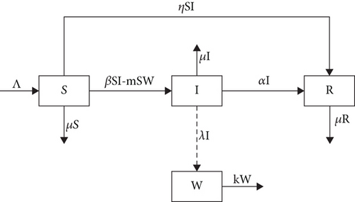
Details are in the caption following the image — Open in figure viewer PowerPoint

Figure 1 indicates that the state changes of the number of rumors in the ignorant, rumor spreader, immune, and communication medium per unit time are as follows.

In the unit time, individuals with a number of Λ enter the population, and these individuals are susceptible. The number of individuals who believe and spread rumors after contacting the communicators is βSI. The number of individuals who do not spread rumors after contacting the disseminator is ηSI. The number of individuals who become communicators under the influence of media coverage effect is mSW. The number of susceptible individuals who have moved out for some reason is μS. So, the number of susceptible individuals varies within a unit time: B − (βSI − mSW) − ηSI − μS.

In unit time, some susceptible individuals who contact and know rumors are partially transformed into communicators. The number of these individuals is βSI. The number of individuals who become communicators under the influence of media coverage effect is mSW. The number of affected individuals converting to the immune individuals is αI. The number of the disseminator who have moved out for some reason is μI. So, the number of spread individuals varies within a unit time: βSI − mSW − αI − μI.

In unit time, some susceptible individuals who contact and know rumors are partially transformed into the immune individuals. The number of these individuals is ηSI. The number of affected individuals converting to the immune individuals is αI. The number of immune individuals who have moved out for some reason is μR. So, the number of immune individuals varies within a unit time: ηSI + αI − μR.

In unit time, the number of rumors spread by the disseminator to the media is λI. Due to the coverage of information in the media, some rumors disappeared. The number of this part is kW. So, the number of rumors in the media varies within a unit time: λI − kW.

Based on the above analysis, the rumor media communication model constructed in this article considering the effect of media coverage is as follows:

(1)

where Λ > 0, α > 0, β > 0, μ > 0, η > 0, k > 0, λ > 0, m < β.

The stability theory of ordinary differential equations is used to analyze the rumor propagation model. Due to the definition of the model, the parameters involved are all nonnegative, and the initial conditions are satisfied:

(2)

3. Model Analysis

Lemma 1. The closed set Ω = {(S, I, R, W) ∈ R⁴, N ≤ Λ/μ, W > 0} is the positive invariant set of model (1).

Proof. It is easy to know that dN/dt = Λ − μN, so N(t) = (N₀ − Λ/μ)e^−μt + Λ/μ, where N(0) = N₀, and then lim_t⟶∞N(t) = Λ/μ. The positive invariant set of system (1) is Ω = {(S, I, R, W) ∈ R⁴, N ≤ Λ/μ, W > 0}.

3.1. The Basic Reproduction Number R₀

The basic reproduction number R₀ [42] represents the expectation of introducing a disseminator into the susceptible population and the number of people that the disseminator can infect in the average cycle of rumor spread. When R₀ < 1, the number of spreaders who can spread during their average spreading period is less than 1; then, the rumors will disappear by themselves. When R₀ > 1, the number of communicators who can spread during their average transmission period is greater than 1, and the amount of rumor communicators gradually increases until they reach the summit. This paper uses the next-generation matrix method to calculate the basic reproduction number R₀ of Equation (1).

Let X = (I, W, R, S)^T, Equation (1) can be written as

Where

(3)

Therefore,

(4)

By calculation, we can get,

(5)

Then, FV⁻¹ is used to represent the next generation matrix:

(6)

Hence, according to reference [42], the basic reproduction number of system (1) is the spectral radius of matrix FV⁻¹ as follows:

(7)

3.2. Existence of Equilibrium

On the basis of the system kinetic Equation (1), we can figure out the equilibrium E = (S, I, R, W). Easily, we find out the positive equilibrium points of system (1) are E₀ = (Λ/μ, 0, 0, 0) and E^∗ = (S^∗, I^∗, R^∗, W^∗), and the rumor-free equilibrium point E₀ invariably exists.

Theorem 1. The equilibrium point E^∗ = (S^∗, I^∗, R^∗, W^∗) exists if R₀ > 1.

Proof. The rumors about system (1) have an equilibrium point that satisfies:

(8)

According to Formula (8), S^∗, R^∗ and W^∗ are represented by I^∗ respectively, and brought into the fifth equation to get

(9)

where,

(10)

It can be obtained by calculation that

(11)

So I^∗ > 0 when R₀ = (Λ(kβ − λm))/(kμ(α + μ)) > 1.

Therefore, E^∗ = (S^∗, I^∗, R^∗, W^∗), where,

(12)

(13)

3.3. Stability of Equilibrium

Theorem 2. The equilibrium point E₀ = (Λ/μ, 0, 0, 0) is locally asymptotically stable if R₀ < 1, m > 0 and .

Proof. The Jacobian matrix of system (1) at E₀ = ((Λ/μ), 0, 0, 0) is

(14)

The characteristic equation of matrix J(E₀) is

(15)

Therefore, the characteristic root corresponding to the characteristic equation of J(E₀) is h₀₁ = h₀₂ = −μ < 0.

Then, we can obtain h² + (k + α + μ − β(Λ/μ))h + k(α + μ − β(Λ/μ)) + λm(Λ/μ) = 0.

When R₀ < 1, m > 0 and

, we can get

(16)

where Δ₁ = (α + μ − k − β(Λ/μ))² − 4[(α + μ − β(Λ/μ)) + λm(Λ/μ)].

According to Routh-Hurwitz stability criterion [39], the equilibrium point E₀ = ((Λ/μ), 0, 0, 0) is locally asymptotically stable if R₀ < 1, m > 0 and .

Theorem 3. The equilibrium point E^∗ = (S^∗, I^∗, R^∗, W^∗) is locally asymptotically stable if R₀ > 1, m < 0, β > α + μ and kβ > λm(1 − α − μ).

Proof. The Jacobian matrix at E^∗ = (S^∗, I^∗, R^∗, W^∗) is

(17)

The characteristic equation of matrix J(E^∗) is

(18)

where,

(19)

It is easy to obtain h₀₁ = −μ < 0.

According to the above characteristic equation:

(20)

where C₁ = μR₀ + (−λm)((α + μ)/(kβ − λm)), C₂ = (−λm)((μR₀(α + μ))/(kβ − λm)).

Let b₃ = 1, b₂ = C₁ + k, b₁ = λmS^∗ + kC₁ + C₂ + A₃, b₀ = λmS^∗(ηI^∗ + μ) + kC₂ + kA₃. Bring the parameter into the expression of b₀, b₁ and b₂ to get

(21)

Then, we can obtain

(22)

And then we can get

(23)

Bring the parameters into the above formula to get: b₂b₁ − b₃b₀ = C₁(C₂ + A₃) − λmS^∗(ηI^∗ + μ) + [kβ − λm(1 − α − μ)]((Λ(C₁ + k))/(μ(α + μ)R₀)).

Hence, when R₀ > 1 and m < 0, we can obtain A₃ = ((Λ(kβ − λm))/(kμR₀))(η + β)I^∗ > 0, C₁ = μR₀ + (−λm)((α + μ)/(kβ − λm)) > 0, C₂ = (−λm)((μR₀(α + μ))/(kβ − λm)) > 0.

Hence, when R₀ > 1, m < 0, β > α + μ and kβ > λm(1 − α − μ), we can obtain b_i > 0(i = 0, 1, 2, 3), b₂b₁ > b₃b₀.

According to the Routh-Hurwitz stability criterion [39], the equilibrium point E^∗ = (S^∗, I^∗, R^∗, W^∗) is locally asymptotically stable if R₀ > 1, m < 0, β > α + μ and kβ > λm(1 − α − μ). Theorem 3 can be proved.

4. Optimal Control

In view of the new rumor dissemination model established abovementioned, in this section, the model is applied to the population in a closed social communication environment. In this paper, two control objectives are proposed. In a certain control time interval, the number of rumor propagators should be reduced, and the number of immune persons should be increased. On the other hand, by controlling the scale of rumor spreading, the cost of human, material, and financial resources will be minimized. Then, the corresponding optimal control problem is studied. Consider that conversion rates β(t) and α(t) have the maximum influence of the rumor propagation model constructed in this paper. Consequently, two proportional constants β and α in the model are transformed into the control variables β(t) and α(t). In this section, for the convenience of calculation, we make β = 1 − μ₁, α = μ₂. Specifically, the control variable μ₁(t) is used to control the proportion of rumor disseminators who are transformed into rumor disseminators after contacting with unknown people. Usually, methods such as publicizing the harm of rumor dissemination and rumor refutation methods are adopted to enhance the public’s ability to identify rumor. In this way, when ignorant people who are not exposed to rumor information are exposed to rumor information, they will consciously identify rumor information and avoid believing and spreading rumor. The control variable μ₁(t) can be understood as the preventive effect, where 0 ≤ μ₁(t) ≤ 1. When μ₁(t) = 1, it means that the preventive effect is 100%. When μ₁(t) = 0, it means that the preventive effect is completely ineffective.

The control variable μ₂(t) is used to control the number of rumor disseminators after taking necessary measures, such as the government issuing relevant laws prohibiting rumor dissemination or designing network rumor information dissemination tracking system and other punishment measures. Hence, there will be corresponding human and material costs in the process of prevention or treatment. Thus, when reducing the scale and controlling the number of rumors, we should not only consider the effect of controlling rumors, but also control the cost. The objective function is defined as follows:

(24)

The optimal control strategy is sought to minimize the objective functional in the control time interval.

Wherein, the variables in (26) satisfy the following state equations:

(25)

and initial conditions

(26)

Here, μ_i(t)(i = 1, 2) is a measurable function, where μ_i(t) ∈ U and 0 ≤ μ₁(t) ≤ 1, 0 ≤ μ₂(t) ≤ 1, ∀t ∈ [0, t_f]. Assume that the starting point of the controlled time zone is 0 and t_f is the end point of the controlled time zone. U is the control allowable set. And the positive parameter c_i(i = 1, 2) is the weight factor, which reflects the control strength and importance of two different control measures.

4.1. Existence of Optimal Control

We use the following theorem to testify the existence of the optimal control tactics for the above-mentioned optimal control problem.

Theorem 4. Consider the control problem with system (1). There exists an optimal control such that

(27)

If the following conditions are met:

(i)
Both control variables and state variables are nonnegative
(ii)
The control admissible set U is convex and closed
(iii)
The integrand in the objective functional is a convex function defined in the admissible set U.
(iv)
The right end of the state system is the linear bounded function of the control variable and the state variable
(v)
The existence of normal numbers d₁, d₂ > 0 and ξ > 1 makes the integrand in the objective functional

(28)

And Equation (28) satisfied

(29)

Proof. Only by verifying that the above five conditions are satisfied, we can prove that the optimal control exists.

Conditions (i)-(iii) are obviously established and only need to prove conditions (iv) and (v).

Given that N(t) = S(t) + I(t) + R(t), state variables have upper bounds N(t), defined by W(t), and it has a positive correlation with I(t), so we also has upper bounds N(t); the following inequality is obtained:

(30)

Hence, condition (IV) is established.

For the last condition , choosing d₁ = min{(c₁/2), (c₂/2)} and any d₂ ∈ R⁺, ξ = 2 can also prove to be satisfied.

4.2. Optimal Control Strategy

The extended Hamiltonian function with penalty term is defined as follows:

(31)

where ω_ij(t) ≥ 0 is a penalty operator, which satisfies

(32)

Theorem 5.

Let S(t), I(t), R(t), and W(t) be optimal state solutions with an associated optimal control for the optimal control problem. Then, there exist adjoint variables λ_i(i = 1, 2, 3, 4) satisfying

(33)

With transversal conditions

(34)

Moreover, the expression of the optimal control pair

(35)

Proof. On the basis of Pontryagin’s maximum principle, we can get the covariate system pass through calculating the derivative of each state variable to Hamilton operator. The synergetic system is

(36)

The definite solution condition of the co state system is

(37)

Then, we discuss how to get the optimal conditions. Take the derivative of Hamilton operator H with respect to state variable U = (μ₁, μ₂), and set it to 0; it can be seen that

(38)

Solve the optimal control expression from it:

(39)

Firstly, we consider

. For the sake of acquire the final expression of optimum control without penalty terms ω₁₁(t) and ω₁₂(t), using standardization techniques, think over the following three situations:

(i)
On the set , let ω₁₁(t) = ω₁₂(t) = 0, so the optimal control is
(ii)
On the set , let ω₁₁(t) = 0, thus
(iii)
On the set , let ω₁₂(t) = 0, thus And because of ω₁₁(t) ≥ 0, it shows (1/c₁)(λ₂ − λ₁)SI ≤ 0.

In summary, the final expression of optimal control

(40)

In the same way, the final expression of optimal control

(41)

Any optimal control pair must meet the optimal control system. The optimal control system (45) is given as follows:

(42)

where and .

5. Numerical Simulation

In this section, we verify the correctness of the above conclusions through numerical simulation. With reference to the parameter values in relevant literature, the parameter values and optimal control problems in the system (1) established in this paper are numerically simulated by MATLAB. The results of the previous theoretical analysis are verified by numerical simulation, and the sensitivity of the model is analyzed.

5.1. Numerical Simulation of System Stability

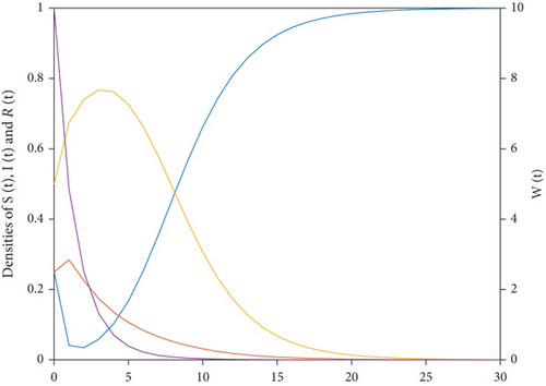
Let Λ = 1, k = 1, β = 0.2, λ = 0.2, m = 0.1, μ = 0.4, α = 0.3, and η = 0.1 and calculate R₀ = 0.6429 < 1, Then, the equilibrium point E₀ of rumor free propagation is stable under different initial conditions. It can be seen from Figure 2 that the stability of E₀ remains unchanged under different initial value conditions.

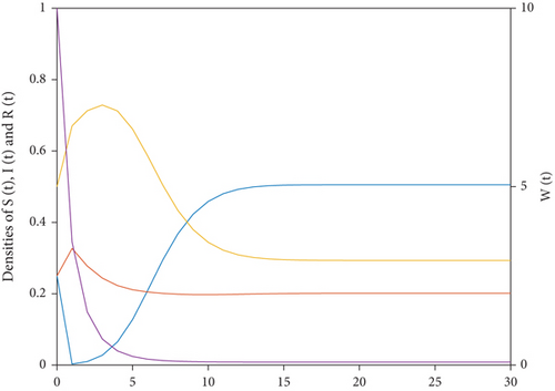
Let Λ = 1, k = 2, β = 0.9, λ = 0.5, m = −0.2, μ = 0.6, α = 0.2, and η = 0.8, and calculate R₀ = 1.9792 > 1, m < 0, β = 0.9 > 0.8 = (α + μ) and kβ = 1.8 > −0.02 = λm(1 − α − μ). The parameter values satisfy the conditions proposed in the third part of Theorem 3. Figure 3 clearly demonstrates the local asymptotic stability of system (1) with respect to the equilibrium point E^∗ under this set of parameter values.

Let Λ = 1, μ = 0.6, η = 0.8, λ = 0.2, and k = 3. When the values of different parameters α, β, m > 0 and m < 0 change, the densities change of S(t), I(t), R(t), and W(t) are shown in Figure 4.

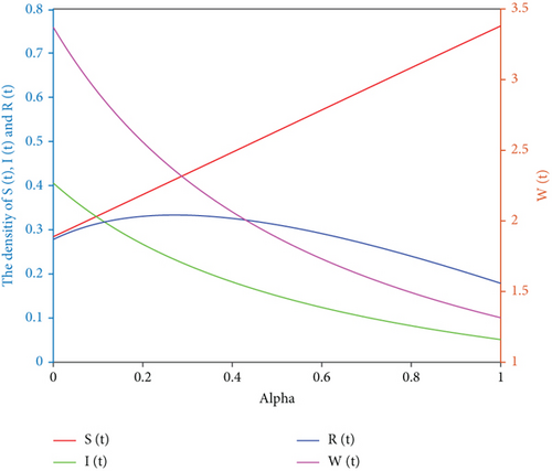
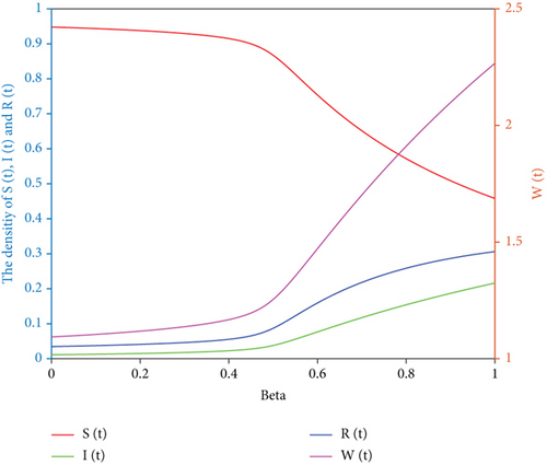
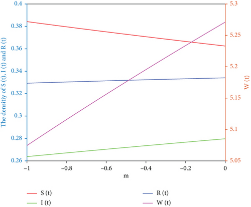
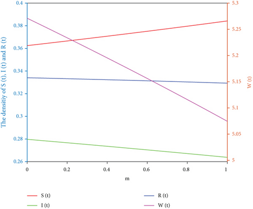
Figure 4 vividly indicates that when α increases, I(t) decreases and R(t) increases. When β increases, S(t) decreases, and I(t), R(t) and W(t) increases, which means increasing the probability of communicators turning into immune ones and reducing the probability of unknown people turning into communicators, which can effectively inhibit the spread of rumors. When m > 0, S(t) increases, and I(t) and W(t) decreases with time, while when m < 0, I(t) and W(t) increase, and S(t) decreases with time. It is not difficult to see from Figure 4 that positive publicity reports help to control the spread of rumors, while negative publicity reports are not conducive to controlling the spread of rumors. However, media reports cannot stop the spread of rumors.

5.2. Numerical Simulation of Optimization System

In this section, according to the method in reference [43], we use the fourth-order Runge Kutta algorithm to simulate the optimization system (45).

The values of simulation parameters in this section are Λ = 1, k = 0.2, λ = 0.9, m = 0.1, μ = 0.65, and η = 0.8, and the initial value is consistent with the previous text.

The weight coefficient in the objective function is difficult to determine, because it is related to the estimation of the cost of two different control strategies, and a large amount of data fitting is usually required to obtain a relatively appropriate trade-off coefficient.

Considering the selection of weight coefficient and the expression of optimal control μ₁ and μ₂, the final weight coefficients are c₁ = 10 and c₂ = 10². It is worth noting that it is difficult to reach the maximum value of control in reality. Therefore, the maximum value control strategy is not considered in numerical simulation.

Remark 1. Figure 5 is the corresponding S(t), I(t), R(t), and W(t) curves under different control strategies when c₁ = 10 and c₂ = 10², i.e.,

(I)
Case without control: μ₁ = μ₂ = 0
(II)
Single control case 1: μ₁ = 0.5, μ₂ = 0
(III)
Single control case 2: μ₁ = 0, μ₂ = 0.5
(IV)
Case of intermediate control: μ₁ = μ₂ = 0.5
(V)
Case of optimal control:

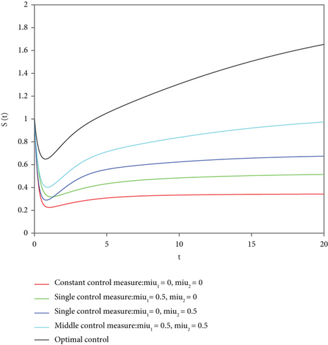
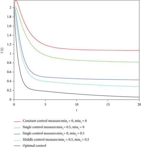
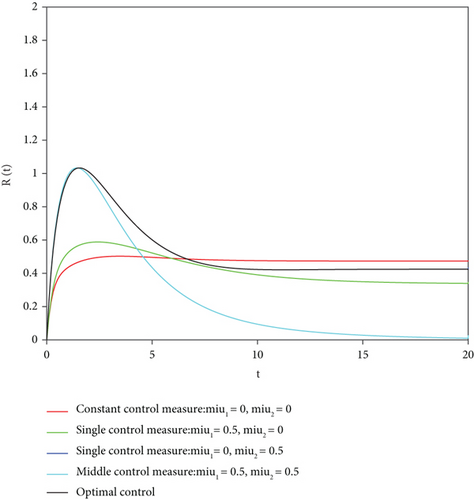
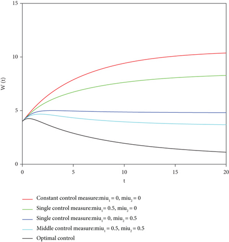
Figure 5 describes the quantity evolution curve of each bin under different control intensities when the weight coefficients c₁ = 10 and c₂ = 10² in the objective function. From the chart, we can see that in the process of reducing the number of communicators and immunizers, the effects of various control strategies should be as below: The optimal control effect is the best, followed by the intermediate value control effect. The effect of single control μ₂ is not as good as that of intermediate value control, but it is obviously better than that of single control μ₁, and single control μ₁ is far better than no control.

6. Sensitivity Analysis of Threshold to Two Control Variables

According to the previously calculated R₀ = ((Λ(kβ − λm))/(kμ(α + μ))), considering the parameter α, we can obtain the partial derivative of R₀:

(43)

This means that when other parameters remain unchanged, if the parameter β increases, the basic reproduction number R₀ also increases. Therefore, the scale of rumor propagation increases. It can be seen from this that if ignorant individuals believe the rumors and spontaneously forward the rumors, it will promote the spread of rumors.

Then, we considered the parameter β, and we can obtain the partial derivative of R₀:

(44)

That means when other parameters remain unchanged, the basic regeneration number is R₀ decreases with the increase of the parameter α, that is, the scale of rumor propagation decreases. It can be seen that if the disseminator loses interest in rumors or no longer disseminates rumor information for other reasons, it will reduce the spread of rumor information and help to control the spread scale of rumor information.

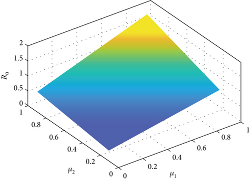
We plotted the three-dimensional relationship between R₀ and the control variables μ₁ and μ₂.

In Figure 6, in order to intuitively see the effect of control parameters on the number of threshold R₀, the three-dimensional curve of R₀ and μ₁ and μ₂ is simulated with MATLAB. Figure 6 shows that the two control variables of R₀ are monotonically decreasing, which means that preventive and punitive measures can better control the spread of rumors. The significance of the control strategy proposed in this paper is further confirmed.

7. Conclusion

Based on the consideration of media reporting effect, this paper established a new rumor propagation model and explored the rumor propagation process under the new communication mode. Firstly, we regard the number of rumors in the media as a variable that changes over time and consider the impact of positive and negative media reports on the spread of rumors. Secondly, for the sake of abate the final cost of suppressing rumor diffusion, the optimal control problem of the model is proposed. Using Pontryagin’s maximum principle, the optimal control solution is calculated in the expected period. Finally, the images of the influence of different parameters on the process of rumor propagation are drawn through numerical simulation.

Compared with the existing literature, we also consider some control strategies, such as deleting rumor information and punishing rumor spreaders, and discuss the optimal control problem to control the scale of rumor propagation and reduce the cost. Numerical simulation shows that under the parameters given in this paper, the optimal control parameter values that meet the constraints can be calculated through quantitative analysis. This method provides a new idea for studying the optimal control of rumor propagation.

Through theoretical analysis and numerical simulation, it shows that the positive publicity and report of the media cannot prevent the spread of rumors, while the negative publicity and report of the media will affect people’s ability to correctly distinguish rumor information, so as to speed up the spread of rumors. In 2011, after the earthquake in Northeast Japan [44], there was a rumor that nuclear radiation would pollute the sea, and the quality of radiation salt led citizens to buy salt crazily. The sensational “doomsday theory” in 2012 led many people to buy all candles in supermarkets, causing unnecessary social panic [45]. Huo and Cheng [46] have described the impact of media coverage and emergency strategies by government on the transmission dynamics of information. That is, after the authorities released the information on eliminating rumors on the official media, the spread of rumors was greatly reduced. Therefore, our theoretical results are consistent with reality.

As a matter of fact, taking the openness and anonymity of the network into consideration, the role of rumor refuter also has an important impact on the process of rumor diffusion. Due to the limited energy, we do not explore the impact of the above factors on the spread process of rumors. It is our future research fields to explore the impact of these influencing factors on rumor propagation.

Conflicts of Interest

The authors declare that they have no known competing financial interests or personal relationships that could have appeared to influence the work reported in this paper.

Authors’ Contributions

Wenqi Pan contributed to the validation, writing-original draft, and writing-review and editing. Yuhan Hu contributed to the conceptualization and visualization. Weijun Yan contributed to the methodology. Ruimiao He contributed to the validation. Libing Wu contributed to the supervision.

Acknowledgments

This work was supported by the Humanities and Social Sciences Research Projects of Education Department of Liaoning Province China (No.2020LNJC11) and the Natural Science Foundation of Liaoning Science and Technology Agency of China (No.2022-MS-356).

Open Research

Data Availability

The data used to support the findings of this study are available from the corresponding author upon request.

References

1 Zhao X. and Wang J., Dynamical model about rumor spreading with medium, Discrete Dynamics in Nature and Society. (2013) 2013, 9, https://doi.org/10.1155/2013/586867, 2-s2.0-84875455157, 586867.
10.1155/2013/586867
Web of Science® Google Scholar
2 Jiang G., Li S., and Li M., Dynamic rumor spreading of public opinion reversal on Weibo based on a two- stage SPNR model, Physica A: Statistical Mechanics and its Applications. (2020) 558, https://doi.org/10.1016/j.physa.2020.125005.
10.1016/j.physa.2020.125005
Web of Science® Google Scholar
3 Yin F., Zhu X., Shao X., Xia X., Pan Y., and Wu J., Modeling and quantifying the influence of opinion involving opinion leaders on delayed information propagation dynamics, Applied Mathematics Letters. (2021) 121, https://doi.org/10.1016/j.aml.2021.107356.
10.1016/j.aml.2021.107356
Web of Science® Google Scholar
4 Aziz-Alaoui M. and Roy P., Deciphering role of inter and intracity human dispersal on epidemic spread via coupled reaction-diffusion models, Journal of Applied Mathematics and Computing. (2021) 66, no. 1-2, 769–808, https://doi.org/10.1007/s12190-020-01450-4.
10.1007/s12190-020-01450-4
Web of Science® Google Scholar
5 Wang M., Hu Y., and Wu L., Dynamic analysis of a SIQR epidemic model considering the interaction of environmental differences, Journal of Applied Mathematics and Computing. (2022) 68, no. 4, 2533–2549, https://doi.org/10.1007/s12190-021-01628-4, 34539297.
10.1007/s12190-021-01628-4
PubMed Web of Science® Google Scholar
6 Daley J. and Kendall G., Epidemics and rumours, Nature. (1964) 204, no. 4963, https://doi.org/10.1038/2041118a0, 2-s2.0-4143136066.
10.1038/2041118a0
PubMed Web of Science® Google Scholar
7 Daley J. and Kendall G., Stochastic rumours, IMA Journal of Applied Mathematics. (1965) 1, no. 1, 42–55, https://doi.org/10.1093/imamat/1.1.42, 2-s2.0-0008904616.
10.1093/imamat/1.1.42
Google Scholar
8 Maki D. P., Maki D. P., Mali D. P., Thompson M., and Thompson M., Mathematical models and applications: with emphasis on the social, life, and management sciences, 1973, Prentice Hall.
Google Scholar
9 Pittel B., On a Daley-Kendall model of random rumours, Journal of Applied Probabilit. (1990) 27, no. 1, 14–27, https://doi.org/10.2307/3214592.
10.2307/3214592
Web of Science® Google Scholar
10 Lefevre C. and Picard P., Distribution of the final extent of a rumour process, Journal of Applied Probability. (1994) 31, no. 1, 244–249, https://doi.org/10.2307/3215250.
10.2307/3215250
Web of Science® Google Scholar
11 Fan K., Zhang Y., Gao S., and Wei X., A class of stochastic delayed SIR epidemic models with generalized nonlinear incidence rate and temporary immunity, Physica A: Statistical Mechanics and its Applications. (2017) 481, 198–208, https://doi.org/10.1016/j.physa.2017.04.055, 2-s2.0-85018642244.
10.1016/j.physa.2017.04.055
Web of Science® Google Scholar
12 Hattaf K., Lashari A., Louartassi Y., and Yousfi N., A delayed SIR epidemic model with a general incidence rate, Electronic Journal of Qualitative Theory of Differential Equatio. (2013) 3, no. 3, 1–9, https://doi.org/10.14232/ejqtde.2013.1.3.
10.14232/ejqtde.2013.1.3
Google Scholar
13 Zhang Y., Xu J., and Wu Y., A fuzzy rumor spreading model based on transmission capacity, International Journal of Modern Physics C. (2018) 29, no. 2, https://doi.org/10.1142/S0129183118500122, 2-s2.0-85043376140.
10.1142/S0129183118500122
Web of Science® Google Scholar
14 Li J., Jiang H., Yu Z., and Hu C., Dynamical analysis of rumor spreading model in homogeneous complex networks, Applied Mathematics and Computation. (2019) 359, 374–385, https://doi.org/10.1016/j.amc.2019.04.076, 2-s2.0-85065542406.
10.1016/j.amc.2019.04.076
Web of Science® Google Scholar
15 Yang Q., Zhang X., and Jiang D., Asymptotic behavior of a stochastic SIR model with general incidence rate and nonlinear LÃ©vy jumps, Nonlinear Dynamics. (2022) 107.
10.1007/s11071-021-07095-7
PubMed Web of Science® Google Scholar
16 Huo L., Cheng Y., Liu C., and Ding F., Dynamic analysis of rumor spreading model for considering active network nodes and nonlinear spreading rate, Physica A: Statistical Mechanics and its Applications. (2018) 506, 24–35, https://doi.org/10.1016/j.physa.2018.03.063, 2-s2.0-85045716690.
10.1016/j.physa.2018.03.063
Web of Science® Google Scholar
17 Li C. and Ma Z., Dynamic analysis of a spatial diffusion rumor propagation model with delay, Adv. Difference Equ.(2015) 2015, no. 1, 1–17, https://doi.org/10.1186/s13662-015-0655-8, 2-s2.0-84948972802.
10.1186/s13662-015-0655-8
Google Scholar
18 Zhu L., Wang X., Zhang Z., and Lei C., Spatial dynamics and optimization method for a rumor propagation model in both homogeneous and heterogeneous environment, Nonlinear Dynamics. (2021) 105, no. 4, 3791–3817, https://doi.org/10.1007/s11071-021-06782-9, 34421220.
10.1007/s11071-021-06782-9
PubMed Web of Science® Google Scholar
19 Xu H., Li T., Liu X., Liu W., and Dong J., Spreading dynamics of an online social rumor model with psychological factors on scale-free networks, Physica A: Statistical Mechanics and its Applications. (2019) 525, 234–246, https://doi.org/10.1016/j.physa.2019.03.037, 2-s2.0-85063675714.
10.1016/j.physa.2019.03.037
Web of Science® Google Scholar
20 Huo L. A. and Ma C., Optimal control of rumor spreading model with consideration of psychological factors and time delay, Discrete Dynamics in Nature and Society. (2018) 2018, 12, https://doi.org/10.1155/2018/9314907, 2-s2.0-85050942447, 9314907.
10.1155/2018/9314907
Web of Science® Google Scholar
21 Laarabi H., Abta A., Rachik M., and Bouyaghroumni J., Stability analysis of a delayed rumor propagation model, Differential Equations and Dynamical Systems. (2016) 24, no. 4, 407–415, https://doi.org/10.1007/s12591-015-0251-0, 2-s2.0-84991402689.
10.1007/s12591-015-0251-0
Google Scholar
22 Zhu L., Liu W., and Zhang Z., Delay differential equations modeling of rumor propagation in both homogeneous and heterogeneous networks with a forced silence function, Applied Mathematics and Computation. (2020) 370, https://doi.org/10.1016/j.amc.2019.124925.
10.1016/j.amc.2019.124925
Web of Science® Google Scholar
23 Yan X. and Ping P., Stability analysis and control models for rumor spreading in online social networks, International Journal of Modern Physics C. (2017) 28, no. 5.
Web of Science® Google Scholar
24 Bianchi P. and Hachem W., Dynamical behavior of a stochastic forward-backward algorithm using random monotone operators, Journal of optimization theory & applications. (2016) 171, no. 1, 90–120, https://doi.org/10.1007/s10957-016-0978-y, 2-s2.0-84979600342.
10.1007/s10957-016-0978-y
Web of Science® Google Scholar
25 Gu J., Li W., and Cai X., The effect of the forget-remember mechanism on spreading, The European Physical Journal B. (2008) 62, no. 2, 247–255, https://doi.org/10.1140/epjb/e2008-00139-4, 2-s2.0-42149184055.
10.1140/epjb/e2008-00139-4
CAS Web of Science® Google Scholar
26 Zhao L., Wang Q., Cheng J., Chen Y., Wang J., and Huang W., Rumor spreading model with consideration of forgetting mechanism: a case of online blogging LiveJournal, Physica A : Statistical Mechanics & Its Applications. (2013) 390, no. 13, 2619–2625.
10.1016/j.physa.2011.03.010
Web of Science® Google Scholar
27 Zhang W., Deng H., Li X., and Liu H., Dynamics of the rumor-spreading model with control mechanism in complex network, Journal of Mathematics. (2022) 2022, 17, https://doi.org/10.1155/2022/5700374, 5700374.
10.1155/2022/5700374
Web of Science® Google Scholar
28 Hu Y., Pan Q., Hou W., and He M., Rumor spreading model with the different attitudes towards rumors, Physica A: Statistical Mechanics and its Applications. (2018) 502, 331–344, https://doi.org/10.1016/j.physa.2018.02.096, 2-s2.0-85042920408.
10.1016/j.physa.2018.02.096
Web of Science® Google Scholar
29 Xu Y., Mei R., Yang Y., and Kong Z., Modeling and analysis of rumor spreading with social reinforcement mechanism, Advances in Mathematical Physics. (2019) 2019, 8, https://doi.org/10.1155/2019/7241021, 7241021.
10.1155/2019/7241021
Web of Science® Google Scholar
30 Hu Y., Pan Q., Hou W., and He M., Rumor spreading model considering the proportion of wisemen in the crowd, Physica A: Statistical Mechanics and its Applications. (2018) 505, 1084–1094, https://doi.org/10.1016/j.physa.2018.04.056, 2-s2.0-85056871199.
10.1016/j.physa.2018.04.056
Web of Science® Google Scholar
31 Qiu L. and Liu S., SVIR rumor spreading model considering individual vigilance awareness and emotion in social networks, International Journal of Modern Physics C. (2021) 31, no. 9, 1–16.
Google Scholar
32 Jain A., Dhar J., and Gupta V. K., Optimal control of rumor spreading model on homogeneous social network with consideration of influence delay of thinkers, Differential Equations and Dynamical Systems. (2019) 2019, no. 1, 1–22.
Google Scholar
33 Yao H. and Zou Y., Research on rumor spreading model with time delay and control effect, Journal of Systems Science and Information. (2019) 7, no. 4, 373–389, https://doi.org/10.21078/JSSI-2019-373-17.
10.21078/JSSI-2019-373-17
Google Scholar
34 Zhang Y., Su Y., Weigang L., and Liu H., Interacting model of rumor propagation and behavior spreading in multiplex networks, Chaos, Solitons & Fractals. (2019) 121, 168–177, https://doi.org/10.1016/j.chaos.2019.01.035, 2-s2.0-85062693576.
10.1016/j.chaos.2019.01.035
Web of Science® Google Scholar
35 Yang L., Li Z., and Giua A., Containment of rumor spread in complex social networks, Information Sciences. (2020) 506, 113–130, https://doi.org/10.1016/j.ins.2019.07.055.
10.1016/j.ins.2019.07.055
Web of Science® Google Scholar
36 Cheng Y., Huo L., and Zhao L., Dynamical behaviors and control measures of rumor-spreading model in consideration of the infected media and time delay, Information Sciences. (2021) 564, no. 3, 237–253, https://doi.org/10.1016/j.ins.2021.02.047.
10.1016/j.ins.2021.02.047
Web of Science® Google Scholar
37 Yu S., Yu Z., Jiang H., and Yang S., The dynamics and control of 2I2SR rumor spreading models in multilingual online social networks, Information Sciences. (2021) 581, 18–41, https://doi.org/10.1016/j.ins.2021.08.096.
10.1016/j.ins.2021.08.096
Web of Science® Google Scholar
38 Zhu L. and Wang B., Stability analysis of a SAIR rumor spreading model with control strategies in online social networks, Information Sciences. (2020) 526, 1–19, https://doi.org/10.1016/j.ins.2020.03.076.
10.1016/j.ins.2020.03.076
Web of Science® Google Scholar
39 Anagnost J. J. and Desoer C. A., An elementary proof of the Routh-Hurwitz stability criterion, Circuits Systems & Signal Processing. (1991) 10, no. 1, 101–114, https://doi.org/10.1007/BF01183243, 2-s2.0-0025956334.
10.1007/BF01183243
Web of Science® Google Scholar
40 Qayyum M., Ismail F., Ali Shah S. I., Sohail M., El-Zahar E. R., and Gokul K. C., An application of homotopy perturbation method to fractional-order thin film flow of the Johnson–Segalman fluid model, Mathematical Problems in Engineering. (2022) 2022, 17, https://doi.org/10.1155/2022/1019810, 1019810.
10.1155/2022/1019810
Web of Science® Google Scholar
41 Qayyum M., Ismail F., Sohail M., Imran N., Askar S., and Park C., Numerical exploration of thin film flow of MHD pseudo-plastic fluid in fractional space: utilization of fractional calculus approach, Open Physics. (2021) 19, no. 1, 710–721, https://doi.org/10.1515/phys-2021-0081.
10.1515/phys-2021-0081
CAS Web of Science® Google Scholar
42 Driessche P. and Watmough J., Reproduction numbers and sub-threshold endemic equilibria for compartmental models of disease transmission, Mathematical Biosciences. (2002) 180, no. 1-2, 29–48, https://doi.org/10.1016/S0025-5564(02)00108-6, 2-s2.0-0036845274, 12387915.
10.1016/S0025-5564(02)00108-6
PubMed Web of Science® Google Scholar
43 Hackbusch W., A numerical method for solving parabolic equations with opposite orientations, Computing. (1978) 20, no. 3, 229–240, https://doi.org/10.1007/BF02251947, 2-s2.0-0000275657.
10.1007/BF02251947
Web of Science® Google Scholar
44 Solove D. J., The future of reputation: gossip, rumor, and privacy on the internet, Social Science Electronic Publishing. (2009) 83, no. 3, 982–992.
Google Scholar
45 Zhao L., Wang Q., Cheng J., Zhang D., Ma T., Chen Y., and Wang J., The impact of authorities' media and rumor dissemination on the evolution of emergency, Physica A: Statistical Mechanics and its Applications. (2012) 391, no. 15, 3978–3987, https://doi.org/10.1016/j.physa.2012.02.004, 2-s2.0-84860531111.
10.1016/j.physa.2012.02.004
Web of Science® Google Scholar
46 Huo L. and Cheng Y., The impact of media coverage and emergency strategies on the rumor spreading, Discrete Dynamics in Nature and Society. (2018) 2018, 14, 4137129, https://doi.org/10.1155/2018/4137129, 2-s2.0-85059886242.
10.1155/2018/4137129
Web of Science® Google Scholar

All articles

Dynamic Analysis and Optimal Control of Rumor Propagation Model with Reporting Effect

Abstract

1. Introduction

2. Rumor Propagation Model with Reporting Effect