1. Introduction

The purpose of this study is carried out the structural analysis of an IS-LM-AS macroeconomic model with adaptive inflation expectations, exploring the presence of a possible local bifurcation. The first contribution of this research lies in the extension of the qualitative analysis of the IS-LM-AS model developed by de La Fuente [1], Gaspar [2], and Shone [3, 4] from the two-dimensional phase space to three-dimensional phase space. The second contribution of this paper consists in analytically and numerically solving the theoretical model developed by Szomolányi et al. [5] for a specific case of the IS-LM-AS macroeconomic model with future inflation expectations. To this end, by adopting specific functional forms for money and goods and services demands, analytical solutions are obtained and the stability analysis of the model is performed. We prove that the model is structurally unstable (presenting a degenerate Hopf bifurcation) when the speed with which economic agents adjust their expectations about future inflation (β) is equal to the inverse of the semi-elasticity of real money demand with respect to the nominal interest rate (h) since the periodic solutions are lost when the adaptive expectations parameter suffer any small change, ceteris paribus. We want to emphasize that the Hopf bifurcation obtained is “non-generic” or “degenerate,” in the sense that the periodic solution only appears when β = 1/h. Indeed, if β < 1/h, all solutions tend to the stationary point when t ⟶ ∞ (the stationary point is asymptotically stable), while if β > 1/h, the stationary point is unstable, more specifically it is a saddle. This distinguishes it from the generic case where from a certain value of the parameter a periodic solution appears, and it does not disappear for values higher or lower than it.

Additionally, the phase portraits of the instantaneous rate of change of the real interest rate, the inflation rate, and the instantaneous rate of change of the inflation rate are numerically simulated in R³ with MATLAB for three asymptotically and locally stable cases and for the degenerate Hopf bifurcation. Finally, our results show that, specifically, in the case of pure conjugate complex eigenvalues, the economy could enter periods of an inflationary/deflationary spiral when the adaptive expectations parameter is of greater magnitude to the inverse of the semi-elasticity of real money demand balances with respect to the nominal interest rate, regardless of its initial state.

2. Material and Methods

In the literature, there are several versions of models based on IS curve, LM curve, and Phillips curve (PC) structures augmented by inflationary expectations or an aggregate supply (AS) function (i.e., IS-LM-PC [AS]) in which the dynamics of said models is incorporated through different assumptions on the adjustment mechanism of expectations, money supply, prices, and potential GDP, among others, and that allow the analysis of the fluctuations of the main macroeconomic variables by means of the quantitative and qualitative tools of ordinary differential equation (ODE) systems or through systems of difference equations. Some of these versions are presented in textbooks [1, 3, 4, 6–9] and others in working papers or scientific articles [2, 5, 10, 11]. (Nozaki (see [11]) performed both theoretical and computational analyses of policy implications of the Kaldor–Phillips business cycle using a nonlinear dynamic IS-LM-PC model along with the Hopf bifurcation theorem in ℝ³. Additionally, Nozaki supplemented the research with theoretical analysis and numerical simulations of a nonlinear dynamic IS-LM model with international trade between two countries in ℝ⁴.)

de La Fuente [1] and Shone [3, 4] developed the qualitative and numerical analysis of a dynamic IS-LM-PC model with adaptive expectations. The qualitative analysis developed by these authors is based on a system of ODEs in ℝ². However, de La Fuente (see [1]) used the real money supply and expected inflation in the qualitative analysis of his model (Altăr [10] analyzed the stability of an IS-LM-AS dynamic model similar to de La Fuente [1] but in discrete time), while Shone (see [3, 4]) used expected inflation and real GDP. In [5], Szomolányi et al. performed a theoretical analysis of an IS-LM-AS model augmented by expectations, finding conditions for its stability and reporting the possibility of cyclical movements of economic aggregates. Likewise, using generic functional forms and modifying their base assumptions, they are able to analyze different economic schools, although they do not carry out a numerical analysis. Gaspar (see [2]), based on the work of Shone [see [4], analyzed economic fluctuations in real GDP and expected inflation with a continuous version of a dynamic linear AS-AD (some discrete and stochastic versions of a dynamic AS-AD model are found in the work of Alpanda et al. [12], Buttet and Roy [13], Lizarazu [14], and Mankiw [15]) model in ℝ², where the AD is obtained from an IS-LM model and the AS (a Lucas-type function) is obtained from a Phillips curve augmented by inflation expectations (PC), finding a “degenerate” Hopf bifurcation when the value of the real money demand sensitivity to changes in the nominal interest rate parameter equals the inverse of the value of the expectations parameter.

In this document, adopting assumptions very similar to those assumed by de La Fuente [1], Gaspar [2], and Shone [3, 4], we extend the qualitative analysis developed by these authors in ℝ² to the three-dimensional phase space. In addition, based on the theoretical model developed by Szomolányi et al. [5], the present paper aims to theoretically and numerically analyze a specific case of the IS-LM-AS macroeconomic model with expectations regarding future inflation.

In concrete, in this article, we examine the possible qualitative changes in the dynamic nature of the model’s phase paths in the neighborhood of its equilibrium point as a consequence of variation in any of its parameters to study the possibility of the presence of a local bifurcation. For this purpose, specific functional forms are adopted for both the demand function for goods and services and the demand function for money. Moreover, for the specific case developed in this article, we assume that the time paths of prices, “P,” and expected inflation, “π^e” (and therefore of real money balances, M/P) are predetermined variables (according to de La Fuente [1], it is assumed that the paths of prices and expected inflation are continuous and, therefore, do not present sudden peaks; in other words, it is assumed that these variables adjust slowly to any changing circumstances), and under a scheme of adaptive expectations about future inflation, the structural stability analysis of the model is carried out in a different but equivalent manner than the analysis performed by Szomolányi et al. [5].

The analytical solutions of the endogenous variables of the model in ℝ³ are obtained for three dynamically and asymptotically stable cases: (i) three different real eigenvalues, (ii) three repeated real eigenvalues, and (iii) one real eigenvalue and two complex-conjugate eigenvalues. Furthermore, using simple programming codes in MATLAB, the phase portraits of the EDOS system governing the dynamics of the modeled economy are obtained through numerical simulations for the three cases analyzed herein, both in ℝ² and ℝ³.

Finally, equal to the results reported by Gaspar [2], when the adaptive expectations parameter (the speed with which economic agents adjust their expectations about future inflation) is equal to the inverse of the semi-elasticity of real money demand with respect to the nominal interest rate, the model presents a degenerate Hopf bifurcation in which periodic solutions are obtained and in which the passage from a stable to an unstable spiral occurs, as the real part of the complex-conjugate eigenvalues changes signs (from negative to positive). However, the linearity of the system of ordinary differential equations (ODEs) governing the dynamics of our model prevents the occurrence of limit cycles (There are dynamic models in the business cycle literature, which use the Poincaré–Bendixson theorem as an analytical tool to verify the existence of limit cycles (Chang and Smyth [16]; Dana & Malgrange [17]; Schinasi [18]; Semmler [19]). However, this theorem cannot be applied to three-dimensional or higher order dynamical systems, but in the literature also, there are several papers that have used the Hopf bifurcation theorem (Poincaré–Andronov–Hopf theorem) to verify the existence of business cycles in nonlinear dynamic models [11, 20–30]).

In Section 2, the model is presented and analyzed, using both quantitative (finding explicit solutions for each case studied) and qualitative (including the detection of local bifurcations) standard approaches in the ODE system literature. The results of numerical simulations are presented for the three asymptotically and locally stable cases and for the degenerate Hopf bifurcation. In Section 3, the results of our theoretical and numerical analysis are briefly discussed. Finally, some conclusions are outlined in Section 4.

2.4. Qualitative Analysis

Let us recall that parameter β appears in equation (6) and gives us an idea of how future inflation expectations are corrected at each t instant proportional to the error that has been made in the forecast. This leads us to consider the following equation:

$$ (72)

as a family of matrices {A_β} indexed by parameter β > 0. We are going to analyze the qualitative behavior of this family of matrices as parameter β changes; for this, we need some definitions and results that can be found in Benazic [31], Lima [32], and Palis and de Mello [33].

We say that matrix A ∈ ℝ^nxn is hyperbolic if and only if all its eigenvalues have nonzero real part. We denote the set of all hyperbolic matrices through Hip(ℝⁿ). Therefore, every hyperbolic matrix is invertible, but there exist invertible matrices that are not hyperbolic.

If A ∈ Hip(ℝⁿ), we can define its index i(A) as the number of eigenvalues with negative real parts (counting multiplicity).

The two matrices, A and B, are topologically conjugate if and only if there exists a homeomorphism h : ℝⁿ⟶ℝⁿ that carries solutions of A in solutions of B, respecting time. Intuitively, two matrices are topologically conjugate by h if and only if the solutions of the linear system of differential equations generated by matrix A are homeomorphic (similar) to the solutions of the linear system generated by B.

We say that a matrix is structurally stable if and only if every matrix B ∈ ℝ^nxn is topologically conjugate to A.

Intuitively, to say that a matrix is structurally stable means that if we perturb it a little bit, then the structure of the solutions of the perturbed system is similar to that of the initial system.

We obtain the following results:

• (i)

  0 ∈ ℝⁿ is a global, exponentially asymptotic attractor if and only if i(A) = n.

• (ii)

  0 ∈ ℝⁿ is a global repellor (sourcer) if and only if i(A) = 0.

• (iii)

  The two matrices A, B ∈Hip(ℝⁿ) are topologically conjugate if and only if i(A) = i(B).

• (iv)

  A is structurally stable if and only if A ∈ Hip(ℝⁿ).

If we go back to the study of family {A_β}, we obtain the following:

• (1)

  If 0 < β < 1/h, then i(A_β) = 3

• (2)

  If β = 1/h, then A_β is not hyperbolic

• (3)

  If β > 1/h, then i(A_β) = 1

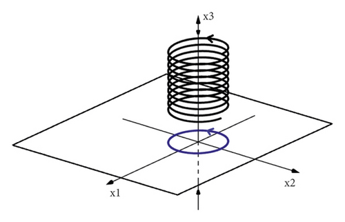
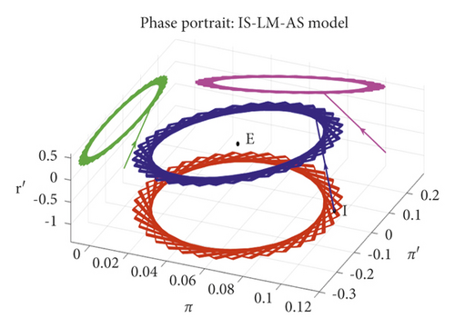
Thus, for parameter β = 1/h, the system ceases to be structurally stable, and therefore, any disturbance, however small, produces a significant change in the configuration of the solutions. In particular, if it is a negative real root and two pure imaginary roots, the solutions of the associated system roll up in a cylinder, having as boundary a circumference in x₁x₂ (see Figure 1).

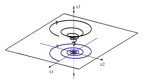
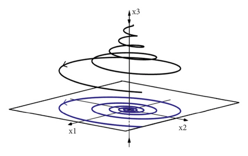
If we take β slightly less than 1/h, then the solutions converge asymptotically to the origin (see Figure 2), while if β is slightly greater than 1/h, then the solutions whose initial value is not on the x₃ axis are divergent (see Figure 3).

In this case, we say that, in parameter β = β₀ = 1/h family, A_β undergoes a Hopf bifurcation of the degenerate type.

2.5. Numerical Simulations

To carry out the numerical simulations of the three asymptotically stable cases and of the degenerate Hopf bifurcation using MATLAB (the MATLAB programming codes used in each simulation can be found in the appendix “A” of this article), we have adopted values for the parameters and exogenous variables of the model based on values, in some cases approximate and in other cases different from those used by other researchers in their scientific papers.

For example, Smith [34] used β = 0.1 in his simulations of a dynamic IS-LM model. Kodera, Sladký, and Vošvrda (see [35]) used ε = 0.4, β = 0.1, and h = 0.06 for their simulations of a dynamic IS-LM-P (rice) MC (Marginal Cost) model. Nozaki (see [11]) used α = 0.3 in simulations of dynamic IS-LM-PC models. Murakami and Zimka (see [26]) used α = 0.3, ε = 1.2, β = 0.12, and h = 0.2 in the computational simulations of a medium-term dynamic Keynesian model. In addition, Moroney (see [36]) reported that, for the period 1980–1993 and for a group of 21 countries with an average GDP growth rate of 2.4% and with an average inflation rate of 2.9%, the average money growth rate amounted to 5.9%. In this paper, we use μ = 0.04 and μ = 0.05.

It is important to highlight that we adopted n = 0 because, otherwise, the real interest rate will tend to be an infinitely negative value in the long run. Finally, the remaining values of the parameters and/or exogenous variables of the model have been assumed to satisfy the assumptions adopted in the model and the signs of the discriminant for each case presented here, as shown in Tables 1–5, respectively.

1. Parameter values and initial and equilibrium values of model variables (Δ = 0).

	Values
Parameters
ψ	1.1
g	3.99
c	0.12
δ = ψ/(1 − c)	1.25
θ = g/(1 − c)	4.534
ε	0.6
h	0.15
μ	0.05
β	0.21
α = 4β(h + εθ)/[θ(1 − hβ)2]	0.56694
n	0
y0p	1
Variables
π0	0.10334
r0	0.0607
$$	0.001326
$$	−0.001679
πE	0.05
rE	0.05513
$$	0
yE	1.00004
YE	2.7183
$$	0
$$	0.04998

2. Parameter values and initial and equilibrium values of the model variables (Δ > 0).

	Values
Parameters
ψ	1.1
g	3.99
c	0.12
δ	1.25
θ	4.534
ε	0.45
h	0.01
μ	0.04
α	0.7
β	0.25
n	0
$$	1
Variables
π0	0.19987
r0	0.00345
$$	−0.0447
$$	0.027
πE	0.04
rE	0.05513
$$	0
yE	1.00004
yE	2.71837
$$	0
$$	0.03998

3. Parameter values and initial and equilibrium values of the model variables (Δ < 0).

	Values
Parameters
ψ	1
g	0.288
c	0.03
δ	1.03092
θ	0.2969
ε	0.01
h	0.1
μ	0.05
α	0.9
β	9
n	0
$$	1
Variables
π0	0.1
r0	0.20312
$$	−0.0017
$$	−1.1017
πE	0.05
rE	0.008
$$	0
yE	1.00718
yE	2.7379
$$	0
$$	0.0435

4. Parameter values and initial and equilibrium values of the model variables (Δ = 0 and β = β₀ = 10).

	Values
Parameters
ψ	1
g	0.288
c	0.03
δ = ψ/(1 − c)	1.030928
θ = g/(1 − c)	0.29691
ε	0.01
h	0.1
μ	0.05
β = β0 = 1/h	10
α	0.9
n	0
$$	1
Variables
π0	0.1
r0	0.1987
$$	0.0052
$$	−1.1071
πE	0.05
rE	0.09
$$	0
yE	1.00421
yE	2.7297
$$	0
$$	0.0462

5. Initial values of the endogenous variables of the model (Δ < 0 and β⋚β₀ = 10).

β values	β = 1	β = β0 = 10	β = 19
Start point	Variables	Values
I1	π0	0.5
	$$	0.005245478
	$$	−0.1
I2	π0	−0.2
	$$	0.005245478
	$$	0.1

2.5.1. Case 1: Null Discriminant (Three Real Eigenvalues: Two of Them Repeated)

Table 1 shows the parameter values adopted for the case of negative real eigenvalues (two of them repeated). In addition, this table shows the initial values and the stationary equilibrium values of the model variables for these parameters.

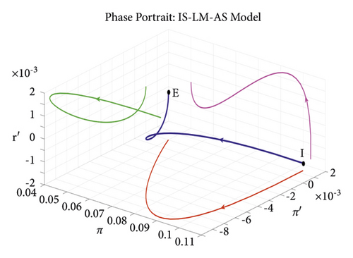
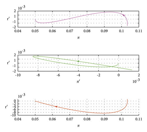
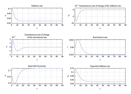
Figure 4, for the values in Table 1, shows the phase path of the economy that at instant “t = 0” starts at $$ and in the long run converges to the steady state “E.” In addition, in this figure, the projections of the phase path in the coordinate planes are observed. Figure 5 shows the ℝ²  projections of the phase path of the economy. Finally, Figure 6 shows the time paths of the interest rate, real GDP, inflation, expected inflation, and the instantaneous rates of change of the interest rate and inflation. This last figure shows that all the paths converge to their respective stationary equilibrium values in the long run in a generally monotonic manner.

2.5.2. Case 2: Positive Discriminant (Three Real and Different Eigenvalues)

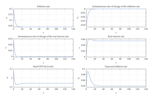
Table 2 shows the parameter values adopted for the case of negative and different real eigenvalues (positive discriminant). This table also shows the initial values and the stationary equilibrium values of the model variables for these parameters.

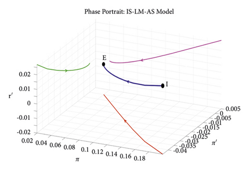
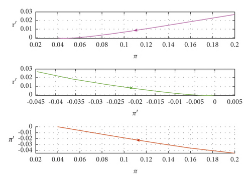
Figure 7, for the values in Table 2, shows the phase path of the economy that at instant “t = 0” starts at $$ and converges to the steady state E in the long term. In addition, the projections of the phase path in the coordinate planes are shown in this figure. Figure 8 shows the ℝ²  projections of the phase path of the economy. Finally, Figure 9 shows the time paths of the interest rate, real GDP (Y = e^y), inflation, expected inflation, and the instantaneous rates of change of the interest rate and inflation. In this last figure, it can be seen that all the paths converge to their respective stationary equilibrium values in the long term, generally in a monotonic fashion.

2.5.3. Case 3: Negative Discriminant (1 Real Eigenvalue and 2 Conjugate Complex Eigenvalues)

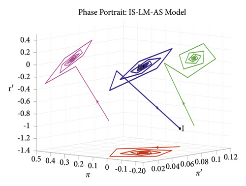
Table 3 shows the parameter values adopted for the case of conjugate complex eigenvalues with negative real part (∆ < 0). In addition, this table shows the initial values and the stationary equilibrium values of the model variables for these parameters.

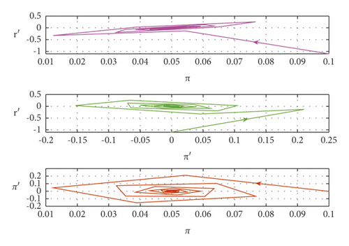
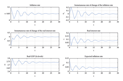
Figure 10, for the values in Table 3, shows the phase path of the economy, which at instant “t = 0” starts at $$ and converges to the steady state E in the long term. In addition, the projections of the phase path in the phase planes are shown in this figure. Figure 11 shows the projections in ℝ²  of the phase path of the economy. Finally, Figure 12 shows the time paths of real GDP (Y = e^y), the interest rate, inflation, expected inflation, and the instantaneous rates of change of the interest rate and inflation. In this last figure, all the paths converge to their respective stationary equilibrium values in the long term in an oscillating fashion.

2.5.4. Degenerate Hopf Bifurcation

Table 4 shows the parameter values adopted for the case of conjugate complex eigenvalues with zero real part (∆ < 0). Additionally, this table shows the initial values and the stationary equilibrium values of the model variables for these parameters.

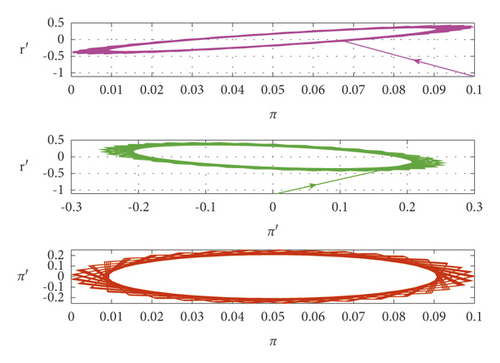
Figure 13 shows the phase path of the economy for the values in Table 4 that at instant t = 0 starts at $$ and oscillates around the steady state E. This figure also shows the projections of the phase path on the coordinate planes. Figure 14 shows the projections in ℝ²  of the phase path of the economy.

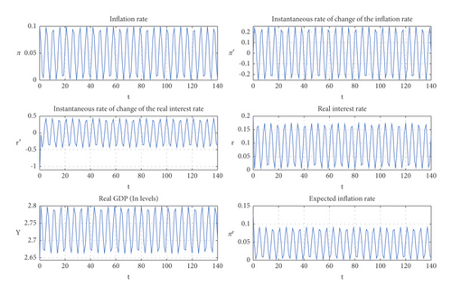
Finally, Figure 15 shows the time paths of the interest rate, real GDP in levels (Y = e^y), inflation, expected inflation, and the instantaneous rates of change of the interest rate and inflation. In this last figure, all the paths oscillate periodically and permanently around their respective stationary equilibrium values.

Moreover, Table 5 shows for the parameter values given in Table 4, the initial values I₁ and I₂ for β less than, equal to, and greater than the Hopf degenerate bifurcation value, that is, for the following values of β : β = 1 < β₀, β = β₀ = 10, and β = 19 > β₀.

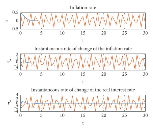
Figure 16 evidences that for the values of the parameters in Table 4, whether the economy starts at I₁ or at I₂ (according to the values given in Table 5), it is found that (i) for values of β < β₀, the phase paths are spirals (red color and blue color curves) converging to the stationary equilibrium E; (ii) for values of β = β₀, the phase paths form closed orbits (purple and yellow colored curves) around the stationary equilibrium point, and (iii) for values of β > β₀, the phase paths are spirals (light blue and green colored curves) divergent with respect to the stationary equilibrium E. Specifically, the economy would enter periods of an inflationary/deflationary spiral in the case where β > β₀ (see top panels of Figures 17 and 18).

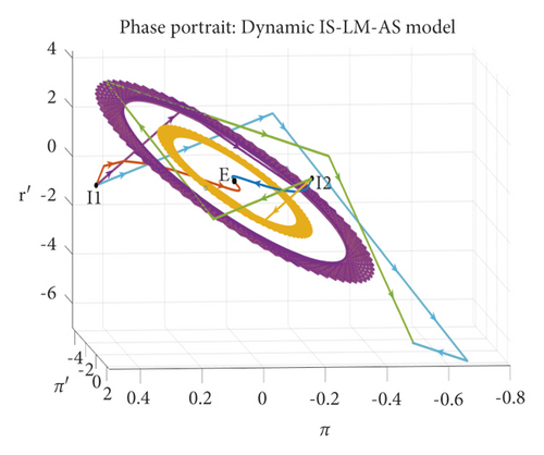
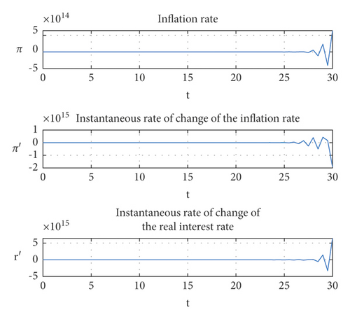
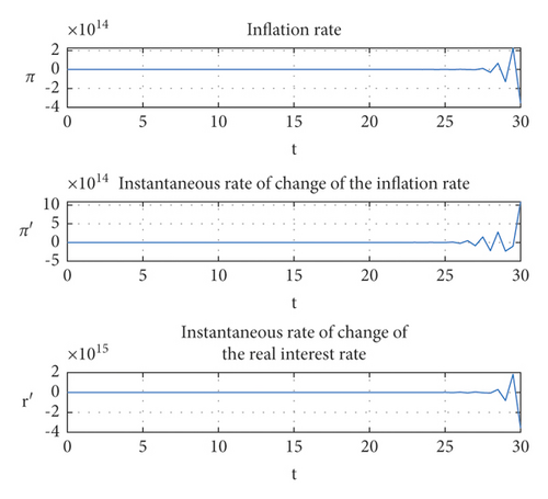
Figure 17 shows the time paths of π, π^′, and r ^′ for the parameter values given in Table 5 for the initial point I₁, given in Table 5, and for β = 1 < β₀ and β = β₀ = 10. It can be observed that for β = 1 < β₀, the paths of π, π^′ and r ^′ converge in an oscillating fashion (albeit with relatively little variability) to their respective stationary equilibrium values. For β = β₀ = 10, the time paths of the three variables oscillate periodically between an upper and a lower bound without permanently converging to the stationary equilibrium but without moving infinitely far from it.

For its part, Figure 18 shows the time paths of π, π^′, and r^′ for the parameter values given in Table 5 for the initial point I₁ in Table 5 and for β = 19 > β₀. In this case, the three paths diverge in an oscillating manner from their respective stationary equilibria.

Figure 19 distinguishes the time paths of π, π ^′, and r ^′ for the parameter values in Table 5 for initial point I₂ in Table 5 and for β = 1 < β₀ and β = β₀ = 10. For β = 1 < β₀, the paths of π, π ^′, and r ^′ converge in an oscillating fashion (albeit with relatively little variability) to their respective stationary equilibrium values. For β = β₀ = 10, the time paths of the three variables oscillate periodically between an upper and a lower bound without permanently converging to stationary equilibrium and without moving an infinite distance away from it.

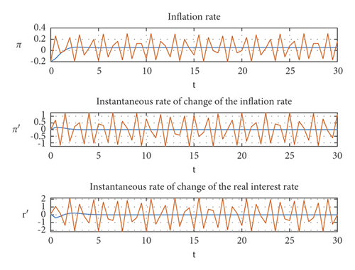
Figure 20 shows the time paths of π, π^′, and r^′ for the parameter values in Table 5, for initial point I₂ in Table 5, and for β = 19 > β₀. In this case, as in the case related to Figure 18, the three paths diverge from their respective stationary equilibria in an oscillating manner.

3. Results and Discussion

According to Vercelli (see [37]), “if a dynamic system is perturbed by an external shock and the perturbed system is equivalent to the original one, it can be considered robust or structurally stable in the sense that it maintains some basic structural characteristics despite the shocks.” For Vercelli (see [37]), “an economic system is dynamically unstable whenever it moves it away from its equilibrium position, it tends to diverge progressively from equilibrium. In this view, the instability of a system depends exclusively on its dynamic behavior with reference to a given equilibrium configuration while the functional and parametric structure of the model remains unchanged.” Moreover, for Vercelli (see [37]), “a system is structurally unstable when as a consequence of a small shock, it undergoes a significant and abrupt change in its structural functions and parameters, which alters the qualitative properties of its dynamic behavior.”

Taking into consideration our theoretical analysis and the result of our numerical simulations for the three cases considered in this article, it can be stated that the model is structurally unstable (presenting a degenerate Hopf bifurcation) when the speed with which economic agents adjust their expectations about future inflation (parameter β is equal to the inverse of the semi-elasticity of real money demand with respect to the nominal interest rate (1/h) because qualitative changes in the dynamic nature of the model’s phase paths, in the neighborhood of its equilibrium point, occur as a consequence of a small variation in the parameter β, ceteris paribus. Nevertheless, paraphrasing to Gabisch and Lorenz (see [38], p. 216), if (economic) reality is stable (in a structural sense), then structurally unstable systems may nevertheless be well-suited to describe actual phenomena as long as the system does not operate in the neighborhood of bifurcation values (degenerate Hopf). However, real economies do not have to be structurally stable.

As pointed out by Vercelli, “the new classical economists apply structurally unstable models (rational expectations models characterized by a saddle point equilibrium) to a reality presented as structurally stable” ([39], p. 54). Furthermore, like Vercelli pointed out, “a model characterized by a saddle point is structurally unstable in the sense that a small disturbance that moves the economy from the convergent trajectory (the stable branch of the saddle) radically modifies the behavior of the system and makes it unstable” ([39], p. 101). However, these types of models are not free from questioning (see, for example, George [40]).

Now, in reference to the literature, it is important to highlight that our model adopts assumptions very similar to those assumed by de La Fuente [1], Shone [3, 4], and Gaspar [2]. However, these researchers carry out a qualitative analysis for systems of first-order ODEs in ℝ². Following the theoretically approach of Szomolányi et al. [5], and through appropriate transformations of variables, we were able to express the dynamics of our model, represented by a system of second-order ODEs in ℝ², through a system of first-order ODEs in ℝ³. This procedure has allowed us to extend the qualitative and numerical analysis of the aforementioned research studies to the spatial domain and, in turn, obtain analytical solutions for the three dynamic and asymptotically stable cases analyzed here.

On the other hand, the results of the theoretical analysis carried out by Szomolányi et al. (see [5]) show that their model presents oscillating solutions when the fulfillment of the next condition is verified: $$ (where “l_r < 0” is the elasticity of the speculative money demand with respect to the nominal interest rate, “l_y > 0” is the elasticity of the transaction money demand with respect to the real output, and “y_r < 0” is the elasticity of the real output with respect to the real interest rate). Furthermore, these researchers found that the solutions of their model are periodic when the condition β = −1/l_r is fulfilled. In our case, our model presents oscillating solutions when α < 4β(h + εθ)/(θ(1 − hβ)²)∧β < 1/h and its solutions are periodic when β = 1/h. Likewise, the structural instability shown by our model is consistent with the possible instability of the model of Szomolányi et al. [5] if the next condition is not met: β < −1/l_r. In our case, in particular, the structural instability occurs when β = 1/h. Finally, as our expected, we have obtained the same result of Gaspar [2] in relation to the emergence of a degenerate Hopf bifurcation in the model when the adaptative expectations parameter match the inverse value of the semi-elasticity of real money demand with respect to the nominal interest rate. Nevertheless, like complement to his theoretically analysis, we also carry out the numerical analysis of this intrinsic characteristic to the model but in ℝ³.

4. Conclusions

In this paper, we have carried out the structural stability analysis in a dynamic IS-LM-AS macroeconomic model based on the work of de La Fuente [1], Gaspar [2], and Shone [3, 4], but extending their bidimensional qualitative analysis to the three-dimensional space phase. In addition, following the work of Szomolányi et al. [5] and through suitable transformations of variables, we were able to characterize the dynamics of our model by means of an ordinary differential equation system in ℝ³. Moreover, we have explored the conditions under which a qualitative change in the dynamical behavior of the model’s phase paths occurs in the neighborhood of its equilibrium point. For this purpose, specific functional forms were adopted for both the demand function for goods and services and the demand function for money.

Therefore, we were able to obtain analytical solutions for three locally and asymptotically stable cases, and we could prove that the model presents a local degenerate Hopf bifurcation when the adaptive expectations parameter β is equal to the inverse of the semi-elasticity of real money demand with respect to the nominal interest rate, 1/h. In addition, we proved both analytically and numerically that for values of 0 < β < 1/h, the system is locally and asymptotically stable (oscillating solutions converging to the stationary equilibrium) (in this case, the locally stable equilibrium of the model guarantees that the time paths of its endogenous variables converge to a new equilibrium in the face of small changes in the values of the model’s parameters), while for values of 0 < β = 1/h, the system is neutral or marginally stable (solutions that oscillate periodically around the stationary equilibrium with relatively constant amplitude). For values of 0 < 1/h < β, the system becomes unstable (solutions oscillating and diverging from the stationary equilibrium), that is, when β is increased from β < 1/h to β > 1/h, the equilibrium point of the system changes its stability because the real part of two of its eigenvalues becomes positive. However, the linearity of our model with respect to its endogenous variables eliminates the possibility of the occurrence of a limit cycle.

Taking into consideration our results, it can be stated that the model is structurally unstable when β = 1/h because the periodic solutions are lost when β undergoes some small change, ceteris paribus. Moreover, our simulations show that, specifically, in the case of pure conjugate complex eigenvalues (with zero real part), the economy could enter periods of an inflationary/deflationary spiral in the case where β > β₀, regardless of its initial state. In addition, notably, there are different configurations that are not analyzed in this paper for which the solutions of the model diverge from the stationary equilibrium (for cases in which all eigenvalues have a positive real part or for cases in which at least one of them has a positive real part and at least another one has a negative real part).

Finally, as a potential line of future research, the option of using functional forms that incorporate nonlinear elements into the model remains open so that it is possible to analyze under what circumstances a single limit cycle could arise, which would allow the endogenous representation of the permanent periodic fluctuations that characterize the cycle of the main economic aggregates.

On the other hand, in recent years several studies on IS-LM business cycle models with time delay have appeared (see [22–24, 41–43]). The qualitative study of the system of functional (delay) differential equations shows that the finite lag may give rise to a wide variety of dynamic behaviors. An important scenario arising from the analysis is the existence of limit cycles generated by sub-critical and supercritical Hopf bifurcations. In [30], the business cycle (BC) is described by a delayed time-fractional-order model (DTFOM) with a general liquidity preference function and an investment function. Fractional-order delayed systems, also appears in other areas such as neural networks (Huang et al. [44], Xu et al. [45], Xu et al. [46], and Xu et al. [47]), bank data (Xu et al. [48]), and eco-epidemiological models (Wang et al. [49]). In all these models, it is important to study stability and propose control strategies to Hopf bifurcations.

In that order of ideas, another line of future research is to consider dynamic IS-LM-AS models with delay and to analyze their stability. There is very little literature on this subject.

Conflicts of Interest

The authors declare that they have no conflicts of interest.