[Retracted] Prediction of Transmission Line Icing Using Machine Learning Based on GS-XGBoost
Abstract
In recent years, data have shown that transmission line icing is the main problem affecting the operation of power grids in bad weather; it greatly increases operating costs and affects people’s lives. Therefore, the development of a calculation method to predict the risk of ice on transmission lines is of great importance for the stability of the power grid. In this study, we propose a maximum mutual information coefficient (MIC) and grid search optimization extreme gradient boosting (GS-XGBoost) transmission line ice risk prediction method. First, the MICs between the ice thickness and the precipitation, wind speed, wind direction, relative humidity, slope, aspect, and elevation characteristic factors are calculated to filter out the effective features. Second, a grid search method is used to adjust the hyperparameters of XGBoost. The resulting GS-XGBoost model builds a prediction system based on the best parameters using a training set (70% of the data). Finally, the performance of GS-XGBoost is evaluated using a test set (30% of the data). For multiline, cross-regional icing data, our experimental results show that GS-XGBoost outperforms other machine learning methods in terms of accuracy, precision, recall, and F1 score.
1. Introduction
Yunnan Province is located at low latitudes and high altitudes, and it has a unique geography that includes rolling mountains and crisscrossing rivers. The cold air from the polar region enters Yunnan after being blocked by the Qinghai–Tibet Plateau, forming the Kunming Stationary Front in northeastern and eastern Yunnan Province, with significant frontal inversion, often forming freezing weather [1]. Qujing and Zhaotong, located in the Kunming Static Line, are the areas in Yunnan that are hardest hit by icing on transmission lines. After icing occurs, the load on a line will increase, and this can lead to excessive sagging and ice ballast jumps, among other undesirable phenomena [2]. The ground line and the same tower erected wire is very easy to short-circuit discharge accidents, and even guide, ground now broken line, inverted tower and other accidents, triggering power grid blackouts [3]. These events seriously threaten the safe operation of the power grid and cause huge economic losses. Effective prediction of transmission line icing provides a convenient way to judge the icing state of power lines, and it can also provide early warnings and a basis for timely deicing operations to ensure the safe and stable operation of the power grid [4].
To solve the problem of transmission line icing and maintain the safety and stability of the power system, scholars have conducted in-depth research to find ways to understand the icing situation at any given time and reduce the occurrence of catastrophic events caused by line icing. Three main types of ice prediction models have been established: physical models, statistical models, and intelligent prediction models.
In terms of physical models, researchers have spent decades establishing calculation models from different perspectives, proposing classical models that take external factors into account, focusing on changes in mass, density, and shape during icing growth [5]. These include the Lenhard model, Chaine–Skeates model, Kuroiwa model, Imai model, Goodwin model, and the McComber–Govoni fog ice cover mathematical calculation model, which provide a reliable theoretical basis for predicting the icing state of power lines [6–11]. These mathematical models of transmission lines provide the most accurate theoretical basis for establishing the true icing state. However, physical models are limited in their practical applications because some of the external factors required for these mathematical models need to be obtained under laboratory conditions and are difficult to measure in real environments.
Statistical models do not consider physical processes, and the most critical part of statistical models is the need for a large amount of historical data. This large amount of data may lead to a rapid increase in computational cost. Wang et al. [12] performed statistical analysis based on ice cover data and found that the ice cover thickness is time-dependent and can be modeled as a time-increasing ice cover prediction. Wang et al. [13] used multiyear ice cover extremes estimated based on the GEV extreme value distribution and found good applicability in both light and heavy ice cover areas. Zhao et al. [14] established a multivariate gray prediction model for icing thickness based on statistics of icing thickness, ambient temperature, and wind speed. Nonetheless, physical and statistical models are not appropriate to solve nonlinear, complex, diverse, and high-dimensional problems [15, 16].
Intelligent prediction models have been proposed by researchers using different representative data. Such approaches include back-propagation (BP) neural networks [17] and support vector machine (SVM) models [18]. Since neural networks can easily fall into local optimal solutions [19], researchers have adopted various strategies to optimize them. Liu et al. [20] proposed a T–S fuzzy neural network to predict icing levels while solving the local optimization problem. Du et al. [21] developed a genetic algorithm (GA) to optimize the prediction model of a BP neural network, and this effectively improved the prediction accuracy. In contrast to neural networks, SVMs do not need to collect a large number of samples, but there are still some problems in their practical application. Several key parameters of SVMs need to be determined according to practical problems. Various optimized and improved SVMs have been proposed, such as the least-squares support vector machine (LS-SVM) [22], wavelet support vector machine (W-SVM) [23], and weighted support vector machine regression (WSVR) [24]. Ma and Niu [25] proposed the fireworks algorithm combined with a weighted least-squares support vector machine (W-LSSVM-FA) for SVM for an icing prediction system and selected appropriate input features to eliminate redundant effects. Niu et al. [26] predicted icing using a combination of AdaBoost and a least-squares wavelet SVM (AdaBoost-LS-WSVM).
Since there are many factors affecting transmission line ice cover and ice cover formation is a nonlinear process, machine learning techniques have been widely and reliably applied in ice cover prediction with high accuracy [20, 26]. In addition to the abovementioned algorithms, extreme gradient boosting (XGBoost) is a popular decision tree-based supervised learning algorithm proposed by Chen and Guestrin [27]. XGBoost is a variant of the gradient lifting method (GBM) [28], which is aimed at improving computational efficiency and flexibility and showing good prediction performance in many fields. To the best of our knowledge, the XGBoost algorithm has not yet been used to predict the risk of transmission line icing.
The icing load of transmission lines will affect the normal operation cycle of equipment, so it is necessary to predict the risk level for line icing. The load state of transmission lines can provide a reference for deicing, resulting in earlier interventions and saving time. In this paper, icing data is classified according to the national icing grade distribution standard, and the maximum mutual information coefficient (MIC) is used to analyze the relevant factors and filter the characteristic factors in the dataset. XGBoost uses the optimal parameters of a grid search combined with a filtered dataset for ice risk-level prediction, providing better adaptability and higher prediction accuracy. This hybrid model can effectively deal with icing data and provide perfect service in the operation of a power grid.
2. Materials and Methods
In Yunnan, the problem of power grid icing is particularly prominent in winter and spring in Qujing and Zhaotong. The icing data recorded by Yunnan power grid from January 1, 2015 to December 30, 2019 were used as an example to establish a prediction model. The specific dataset is shown in Table 1.
| Minimum temperature | Wind direction | Speed | Precipitation | Relative humidity | Elevation | Slope | Aspect | Icing thickness |
|---|---|---|---|---|---|---|---|---|
| 8.89 | 7 | 4.87 | 0.80 | 87.68 | 1355 | 4.84 | 163.30 | 0 |
| −0.10 | 5 | 3.48 | 1.45 | 93.75 | 2153 | 9.37 | 335.32 | 1 |
| … | … | … | … | … | … | … | … | … |
| −2.18 | 4 | 4.07 | 0.27 | 85.37 | 2084 | 1.77 | 246.80 | 3 |
| −1.76 | 8.00 | 5.24 | 0.12 | 89.22 | 2122 | 4.60 | 310.91 | 4 |
The dataset consists of two main parts: (1) meteorological and geographic data comprising eight characteristic factors: minimum temperature, wind speed, wind direction, precipitation, relative humidity, slope, slope direction, and elevation and (2) ice thickness. Due to the long period and wide regional span of this dataset, all ice cover data were recorded manually, and there are therefore some data inaccuracies. In this work, we adopted the classification of ice cover thickness level to predict the risk of ice on the power grid, in which the ice cover levels are divided according to the zoning range criteria of the national technical guidelines for ice area distribution mapping, as shown in Table 2. Therefore, the dataset used in the experiments contains two parts: the ice cover risk level and the feature factors, which comprise meteorological and geographical data. After data cleaning, there were 109,373 data points, and these were divided into a training set (76,561) and a test set (32,812) in the ratio 7 : 3.
| Ice thickness range (mm) | Level |
|---|---|
| 0 | 0 |
| (0, 5] | 1 |
| (5, 10] | 2 |
| (10, 20] | 3 |
| (20, 30] | 4 |
| (30, 40] | 5 |
2.1. Building the Prediction Model
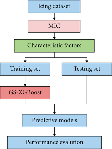
In response to the above problem, we propose to predict the risk level for transmission line icing so that workers can quickly respond to severely problematic areas and deice them in a timely manner. Lower risk-level areas can adopt manual deicing or natural deicing according to the different loads of the transmission lines in different regions. This will reduce labor costs and maintain the normal operation cycles of equipment. Our prediction model is constructed as shown in Figure 1. First, the ice thickness is classified according to the zoning scope of the technical guidelines for drawing the national ice distribution map, and the data is cleaned. Second, the MIC is applied to the relevant characteristic factors of ice cover for correlation evidence analysis and screening of the characteristics. Third, 70% and 30% of the icing data points are selected as the training and test sets, respectively. Fourth, fivefold cross-validation (CV) and grid search are used to adjust the model parameters. Finally, XGBoost fits the prediction model based on the optimal parameters found in the training set. In this work, comparisons were made with several other models to establish the accuracy and suitability of the proposed model.
2.2. Maximum MIC
2.3. XGBoost Algorithm
XGBoost constructs the decision tree based on the difference obtained from Equation (15), and by traversing the value cases of all features, a node is selected for splitting when the difference between the value before and after the loss function reaches the maximum value. In addition, the difference in the loss function before and after splitting must be positive, which can be considered to play the role of preshearing.
2.4. Grid Search- (GS-) XGBoost
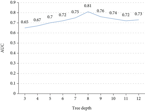
Grid search is a common exhaustive parameter adjustment method. This paper uses tenfold cross-validation to tune hyperparameters. Given a series of hyperparameters, a grid search exhaustively traverses all their possible combinations and selects the optimal set. This method can find the optimal solution among all possible solutions. It is applied to optimize several key superparameters in XGBoost and optimize the performance of the model. The specific meaning and tuning ranges of the superparameters are shown in Table 3. The AUC value predicted by the model increases as the tree depth increases. When the tree depth is 8, the AUC value of the model is the largest, and as the tree depth continues to increase, the AUC value of the model begins to decrease and tends to be stable. So this paper sets the depth of the tree to 8, and the specific index optimization diagram is shown in Figure 2.
| Algorithm | Hyperparameter | Meanings | Search range | Optimal value |
|---|---|---|---|---|
| XGBoost | Learning_rate | Shrinkage coefficient of each tree | [0.1, 0.6] | 0.6 |
| Subsample | Subsample ratio of training samples | [0.8,0.9] | 0.9 | |
| Colsample_bytree | Subsample ratio of columns for tree construction | [0.6,0.8] | 0.8 | |
| Max_depth | Maximum depth of a tree | [3, 8] | 8 |
2.5. Correlation Analysis
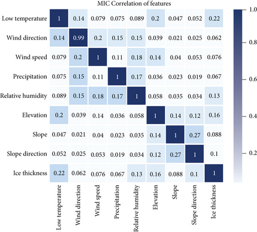
The MIC was applied to analyzing the correlations of features in the dataset, and some of the feature factors with weak correlations were removed. The generated coefficients will indicate whether a feature factor is important for the formation of ice cover on transmission lines. In this paper, the MICs were calculated for the following parameters in the dataset: daily minimum temperature, maximum wind speed and direction, maximum wind speed, precipitation, relative humidity, slope, slope direction, and elevation. The resulting coefficients are shown in Figure 2, in which it can be seen that the daily minimum temperature and relative humidity are important factors in the formation of ice cover. These are followed by altitude, with a coefficient of 0.22, which indicates that this geographical factor is also one of the conditions leading to ice. Wind speed, wind direction, and precipitation are less correlated with the other factors. The influences of slope and slope direction on the ice cover in this application area are relatively weak.
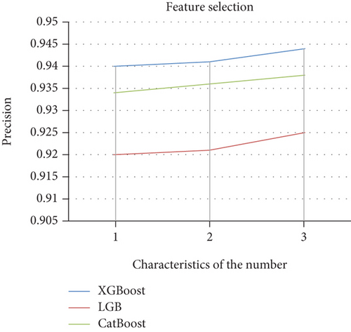
The two feature factors with the smallest MIC coefficients (slope and slope direction) were deleted through multiple comparison tests, demonstrating that the MIC can be used to screen invalid feature factors more accurately, as shown in Figure 3. In the plot in Figure 3, the horizontal coordinate indicates the number of features removed, with 1 indicating a factor that removes the smallest MIC coefficient (slope) and 2 indicating that two feature factors (slope and slope direction) that remove the smallest coefficient. Due to the robustness of their algorithms, XGBoost, LightGBM, and CatBoost exhibit no major changes in accuracy when some features are removed; however, after removing slope and slope direction, the accuracy is higher than when these features are not removed. As can be seen from Figure 3, the algorithm used in this paper always performed better than the others with which it was compared. In addition to the three algorithms mentioned above, a feature selection comparison experiment with a plain Bayes algorithm was carried out, and the accuracy was only 59% without removing features and improved by about 9% after removing slope and slope direction, and 72% after removing slope and slope direction. The schematic diagram of feature selection is shown in Figure 4.
2.6. Evaluation Indicators
Accuracy, precision, recall, and F1 score were used as the evaluation indexes for icing risk in this paper. Accuracy is the proportion of correct predictions, precision assesses the accuracy of the detection of positive examples, and recall rate evaluates the recall rate for real positive examples. The basic classifiers are shown in Table 4.
| Relevant | Not relevant | |
|---|---|---|
| Retrieved | True positive (TP) | False positive (FP) |
| Not retrieved | False negative (FN) | True negative (TN) |
In the table, TP indicates a positive examples classified as a positive examples (correct classification), FP indicates a negative examples classified as a positive case (misclassification-misclassification of negative samples as positive samples), FN indicates a positive example classified as a negative case (misclassification-misclassification of positive samples into negative samples), and TN indicates originally negative example that were classified as negative examples (correct classification). The values of P = TP + FP indicates all samples classified as positive, and N = FN + TN indicates all samples classified as negative.
3. Results
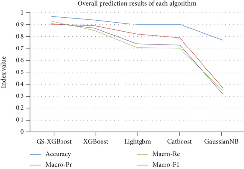
The results of the GS-XGBoost algorithm were obtained on the test set and compared with the evaluation metrics of the untuned XGBoost, LightGBM, CatBoost, and GaussianNB results. As shown in Table 5, the evaluation indicators were calculated according to Equations (16)–(19). The results show that XGBoost had good prediction effect on icing risk level without tuning the superparameters, and the accuracy of XGBoost was the highest, reaching 0.94. The accuracies of LightGBM and CatBoost were both 0.90, but their recall rates were 0.71 and 0.70, respectively. According to the confusion matrix, the results were not very good in some categories. The accuracy of the GaussianNB prediction reached 0.77, indicating that the algorithm is not suitable for icing risk prediction. After hyperparameter adjustment of XGBoost through a grid search, the results were significantly improved. However, the samples of risk prediction of icing risk level were not balanced, and the accuracy rate reached 0.97. The other four indicators were all above 0.90, indicating that the prediction results of our model were more accurate. The accuracy indicators of the five models are shown in Figure 5.
| Model | Accuracy | Macro-Pr | Macro-Re | Macro-F1 |
|---|---|---|---|---|
| GS-XGBoost | 0.97 | 0.90 | 0.93 | 0.91 |
| XGBoost | 0.94 | 0.89 | 0.85 | 0.87 |
| LightGBM | 0.90 | 0.82 | 0.71 | 0.74 |
| CatBoost | 0.90 | 0.79 | 0.70 | 0.73 |
| GaussianNB | 0.77 | 0.37 | 0.35 | 0.32 |
4. Discussion
In this work, the MIC was used to analyze the correlation of ice cover-related feature factors. The most important factors were found to be daily minimum temperature and average relative humidity, and the weakest correlations were found with the slope and slope direction; these features were thus removed by comparative tests. It was proposed that the GS-XGBoost model should be applied to solve the transmission line ice risk problem. Transmission line ice datasets for Qujing and Zhaotong cities in Yunnan Province for the past five years were selected for empirical analysis.
To solve the transmission line ice load problem, the MIC, combined with the GS-XGBoost intelligent algorithm proposed in this paper, can be used to predict the risk level of transmission line icing. This model can be used conveniently by relevant departments to establish the icing load on transmission lines at any given time, and they can then take corresponding measures to reduce the damage and inconvenience to equipment or residents’ lives. Compared with previous studies, the grade prediction of icing in this paper is slightly different from the prediction of icing thickness; it can directly predict the risk state of icing on transmission lines, and this allows relevant departments to take timely action. The transmission lines in different regions will be subject to different icing-related conditions, and the datasets will not be identical. In this work, the MIC was calculated between the icing thickness and collected relevant factors. This allows calculation of correlation coefficients with lower complexity and higher robustness. The GS-XGBoost method showed good performance in predicting ice risk levels.
It is clear that the aggregation of and relationships between real-time meteorological and geographical data and icing monitoring need to be further studied, and the research in this paper is a useful initial exploration. This work provides scientific guidance for predicting the icing risk level in advance of any problems, and it allows appropriate and timely ice-melting measures to be taken.
Conflicts of Interest
The authors declare that there is no conflict of interest regarding the publication of this paper.
Open Research
Data Availability
This article contains data to support the results of this research. Some data cannot be provided because it involves the coordinate data of power grid poles.


