In order to improve the classification effect of the 3D CAD model, this paper combines the knowledge recognition algorithm of convolutional neural network to construct the 3D CAD model classification model. Moreover, this paper analyzes the application of the convolutional neural network algorithm in the classification of 3D CAD models, improves the knowledge recognition algorithm, and builds the basic structure of the convolutional neural network. In addition, this paper builds an intelligent recognition model with the support of the improved algorithm, designs experiments to verify the effect of this paper, and draws a visual display statistical graph based on the statistical test results. Through experimental research, it can be known that the 3D CAD classification model based on the knowledge recognition algorithm of convolutional neural network proposed in this paper can effectively improve the classification effect of the CAD model.

1. Introduction

The traditional 3D model classification method is to manually extract the model representation and then complete the classification of the 3D model. From the perspective of its characterization model, it can be divided into two categories. The first category is to directly extract the corresponding descriptors from the model itself, such as generating descriptors on a voxel grid or polygonal grid. The second category is the use of view-based descriptors to express models. The principle is to first project the 3D model to obtain a series of useful two-dimensional image information [1]. The above method is an extraction method designed manually, which has problems such as strong subjectivity, poor practicability, and complex extraction process. Therefore, some scholars have begun to consider new ways. With the development of computer hardware, the concept of deep learning has emerged. Its principle is to transform the input signal layer by layer, transform the sample feature representation into a new high-level feature representation, and autonomously learn the hierarchical feature representation of the sample. Compared with the shallow learning model, the extracted model features are more abstract, and the classification and retrieval of the model with this abstract feature is more in line with the human visual system [2].

Product design and manufacturing based on 3D CAD models have many excellent characteristics, such as visualization, virtualization, and digitization. These characteristics make it an indispensable basic carrier in the process of product design and development for designers. Nowadays, 3D CAD models have become the mainstream auxiliary means of China’s manufacturing industry [3].

Through investigation and statistical analysis, it is shown that, in the process of developing new products, about 40% of the designs will use existing components in the past, and nearly 40% of the designs will be improvements to existing designs. 20% of the designs are based on new ideas. Therefore, quickly and accurately classify existing 3D CAD models and return back similar designs according to user needs so that designers can reuse models efficiently. This not only saves product production costs but also effectively reduces development time costs and improves design efficiency. Based on the above, the 3D CAD model retrieval technology came into being. It can realize the effective and rapid classification of product CAD model resources by enterprises and provide a powerful means of expenditure for the reuse of various product design processes. Since the classification of industrial CAD models requires a wealth of professional domain knowledge, in most cases, the classification work is mainly carried out by engineers. The process is very time-consuming and labor-intensive, and such a monotonous and lengthy manual operation will cause frequent misclassification of models in the classification process. Many scholars have conducted research on the model classification process and have proposed many methods of automatic classification using computers. Traditional automatic classification algorithms extract feature descriptors by designing a certain feature description extraction algorithm by the user and use machine learning algorithms to complete the automatic classification of the model. However, due to the complexity of the three-dimensional model itself, this user-designed feature descriptor extraction algorithm is difficult to completely and accurately capture the feature information of the three-dimensional model, and its expression ability is limited; shallow machine learning is due to insufficient training set and computing power. The limitation of the expression effect of functions that are inherently difficult to solve has caused their application to relatively difficult classification problems to be restricted to a certain extent.

This paper combines the knowledge recognition algorithm of convolutional neural network to construct the 3D CAD classification model, improve the classification effect of 3D CAD model, and enhance the work efficiency of industrial design.

2. Related Work

Literature [4] uses machine learning algorithms to automatically classify entity models. This method converts the entity model into a histogram through the shape distribution and then uses the kNN algorithm for classification, but the accuracy of the classification is not high. Then IP uses surface curvature and SVM to classify the CAD model. The four curvatures of the model are used to calculate into vectors, and the classification is carried out by support vector machine. The experimental results show that the classification result of the smallest curvature is the most ideal. Literature [5] combines support vector machine with 3D model, a semisupervised classification 3D model. In the reform work, each input data is represented by a mixture of three eigenvectors in order to express the three-dimensional body from different angles. This method tested 218 three-dimensional models and achieved a relatively low error rate. Literature [6] proposes an automatic selection of appropriate descriptors to classify 3D models. This model combines shape distribution descriptors, sparse theory, and spectral clustering to achieve the purpose of classifying 3D models.

Literature [7] starts from the surface of the model by defining the attributes of the surface and the type of the intersection edge between the surface and the surface, forming a matrix, constructing the input vector and uses the multiperceptron learning algorithm to develop a feedforward neural network that can be used in the field of 3D model recognition. Literature [8] uses the Kohonen self-organizing neural network to unsupervised decomposition of the public ground with cross-features and gives feature explanations. This idea is another breakthrough in the recognition of cross-features of neural networks. In this method, the way of competitive learning is that different neurons are sensitive to different features so as to explain the cross-features. But this method sometimes complicates the problem and may cause deadlock.

Literature [9] puts forward a new idea of training deep network, which makes people’s eyes turn back to the neural network, and believes that the artificial neural network structure formed by stacking multiple hidden layers has better feature learning capabilities, and the features extracted through the network can more essentially describe the data, which is more conducive to data classification. It also proposed that deep neural network training will be very complicated in theory and consider using layerwise pretraining to solve it better. These two views are the essence of deep learning. Nowadays, deep learning has been developed by leaps and bounds in applications in many fields. Literature [10] established a huge deep neural network learning model, which has been applied to the fields of speech recognition and image recognition and achieved outstanding results. Literature [11] applies CNNs to handwriting recognition in the MNIST database. Using the local receptive field method to obtain observation features, the obtained features have nothing to do with translation, scaling, and rotation, and the effect of handwriting recognition is extremely ideal. Literature [12] found that deep learning networks can perform better on audio data. Literature [13] found that the representation obtained through deep learning has a better effect on the style classification problem. Literature [14] established a deeper convolutional neural network to deal with the problem of image gridding and achieved the best results so far. Literature [15] uses unprocessed natural images as the input of deep neural network models for unsupervised training. Now, the application of deep learning algorithms is no longer limited to image classification. In a wider range of visual problems, deep learning has had a significant impact, such as face recognition, general object detection, image classification, optical character recognition, and even applied to games. Literature [16] established an empirical evaluation model for video classification based on convolutional neural networks and divided 1 million pieces of YouTube video data into 487 categories. The single frame, two nonadjacent frames, adjacent multiple frames, and adjacent frames of multistage are merged, and the deep convolutional network is used for training. It also pioneered a multiresolution network structure that can increase the speed of convolutional neural network training.

3. Knowledge Recognition of the Convolutional Neural Network

Ω is the set of proposition A; that is, Ω = {A₁, A₂, …, A_n}. The propositions in Ω are finite, complete, and mutually exclusive. All possible combinations of proposition A form the power set 2^Ω2^Ω; that is, 2^Ω = {Φ, {A₁}, …, {A_n}, {A₁ ∪ A₂}, {A₁ ∪ A₂ ∪ A₃}, …}. Under the framework of identification, the combination of any single proposition is called single-point evidence, and the combination of any two or more propositions is called nonsingle-point evidence.

Definition 1. For any proposition A of the power set, this paper defines the mapping m: 2^Ω⟶[0,1], which satisfies the condition of formula (1), which is shown as follows:

()

It is said that m is the probability distribution function on 2^Ω, and m(4) is called the basic probability assignment (BPA) of A, which represents the initial support of proposition A to the source of evidence. If m(A) > 0, then A is called focal element. The function of the probability distribution function is to map any subset A of the identification frame to the interval [0,1] to obtain the value m(A). m(Al) also represents the accurate trust in A, but it is not clear how to assign the trust to the elements of A. However, when A = Q, m(A) represents the remaining part after the trust assignment is performed on each subset of Q, and it is unknown how to assign this part.

Definition 2. For any proposition A, the sum of the basic probability distributions corresponding to all subsets in A is called the Belief function (Bel) of A, which satisfies the condition of formula (2), as shown as follows [17]:

()

Bel(A) is called the trust function or the lower limit function, which represents all the trust in A. Its value is the sum of the basic probabilities of all subsets of A. It is easily obtained from the definition of BPA:

()

Definition 3. For any proposition A, PI(A) represents the degree of trust in A not false, which satisfies the condition of formula (4), as shown as follows [18]:

()

PI(A) is called the likelihood function (Plausibility function, PI), also called the upper limit function, which represents the uncertainty measurement that may hold for A.

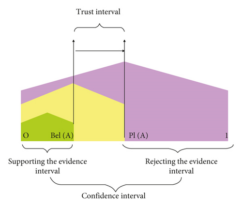
Obviously, Bel(A) and PI(A) have the following relationship: PI(A) ≥ Bel(A), A⊆Ω. The uncertainty of A is represented by PI(A)-Bel(A), and (Bel(A), PI(A)) is called the confidence interval, as shown in Figure 1.

Figure 1 shows that the trust degree Bel(A) is the lower bound estimate of the hypothesis trust degree of proposition A, that is, the minimum value of A’s credibility, which is a pessimistic estimate. Likelihood PI(A) is the upper limit estimate of the degree of confidence in the hypothesis of proposition A, that is, the maximum value of A’s credibility, which is an optimistic estimate. Table 1 shows some common confidence intervals.

Details are in the caption following the image — Open in figure viewer PowerPoint

1. Common confidence intervals.

Evidence interval	Explanation
[1, 1]	Totally true
[0, 0]	Totally fake
[0, 1]	Totally ignorant
[Bel,1], where 0 < Bel < 1	Tends to support
[0.PI], where 0 < PI < 1	Tends to rebut
[Bel,PI], where 0 < Bel ≤ PI < 1	Tend to support and rebut

3.1. Synthesis Rules

We assume that A₁ and A₂ are the two propositions in the identification framework 2; then, m₁(A₁) and m₂(A₂) are the two basic probability distributions on the power set E. According to the DS theory, the fusion rule of the two pieces of evidence m₁ and m₂ is defined as follows:

()

Among them,

. k reflects the degree of conflict of the evidence, called the conflict factor. (1 − k)⁻¹ can avoid assigning the nonzero probability to the empty set when the evidence is combined, called the correction factor. By extension, we assume that there are n propositions on the identification frame Q, and the basic probability distribution is m; i = 1, 2, …, n. The fusion rule for any subset A ∈ Q2 on the power set 2n is shown in the following formula:

()

Among them, .

The mathematical formula of the fusion rule shows that the essence of DS theory is the orthogonal sum of two pieces of evidence. Therefore, it satisfies the commutative law and the associative law.

The commutative law is as follows [19]:

()

The law of associativity is

()

3.2. Decision Rules

After the fusion result is obtained by the combination rule of DS theory, the decision-making judgment is made according to m(A). Common judgment methods include BPA-based methods, Bel function-based methods, and minimum risk-based methods. The method based on BPA is widely used. We set any propositions A and A in the identification framework Q to satisfy the condition of the formula

()

Then, A is the decision result, where z and e are preset thresholds. This value is generally set by the expert system or the worker’s experience value. This paper sets ε₁ = 0.1 and ε₂ = 0.05.

Learning vector quantization (LVQ) neural network is derived from self-organizing competitive network, which concentrates on the advantages of competitive response and supervised learning and makes up for the lack of classification labels of self-organizing network. When a certain vector is sent to the LVQ, the nearest competing layer neuron is activated, and the state is set to 1, the linear output layer neuron connected to the activated neuron is also set to 1, and the others are set to 0l77l. The LVQ neural network structure is shown in Figure 2.

Among them, p is the R-dimensional input vector, S′ is the number of neurons in the competition layer, IW is the connection weight coefficient matrix between the input layer and the competition layer, n is the input of the neurons in the competition layer, a’ is the output of neurons in the competitive layer, LW2 is the connection weight coefficient matrix between the competition layer and the linear output layer, n2 is the input of the neuron in the linear output layer, and a2 is the output of the neuron in the linear output layer.

There are two commonly used algorithms in LVQ networks.

3.2.1. The LVQ1 Algorithm

The LVQ1 algorithm calculates the distance between the initial weight and the input vector, selects the closest competing layer neuron, and activates it, thereby correlating the corresponding linear output layer neuron. If the label of the input vector is the same as the label corresponding to the linear output layer, the network weight is adjusted to the input direction; otherwise, it is adjusted in the reverse direction. The specific steps are as follows [20]:

Step 1. The algorithm initializes the network weight w_ij and the learning rate η(η > 0) randomly.

Step 2. The algorithm sends the input vector to the input layer and calculates the distance d_i.

()

Step 3. The algorithm selects the nearest competing layer neuron. If d_i is the smallest, set the category information of the output layer neuron connected to it as C_i.

Step 4. The algorithm records the category information of the input vector as C_x. If C_x = C_i, use formula (11) to update the weight, as shown as follows:

()

Otherwise, the algorithm adopts formula (12) to adjust the weight.

()

Step 5. The algorithm judges whether it meets the preset termination conditions. If it matches, the algorithm terminates; otherwise, it returns to the second step to continue to update the network weight.

3.2.2. The LVQ2 Algorithm

In the ILVQI algorithm, only one neuron that wins the competition can adjust the weight. In order to improve the classification and recognition rate of the network, LVQ2 introduces the second-winning neuron, and the weights of the winning and the second-winning neuron will be adjusted. The specific steps are as follows:

Step 6. The algorithm sends the input vector to the input layer and calculates the distance.

Step 7. The algorithm selects the closest two competing layer neurons i and j.

Step 8. If ü and j meet the following requirements, then we have the following:

①
Neurons i and j correspond to different labels;
②
The distances d and d between neurons i and j and the current input vector meet the requirements of

()

Among them, p is the width of the window close to the midsection plane of the two vectors that the input vector may fall into, generally taking 2/3 up and down. Then, we have the following.

If the label C_i corresponding to the neuron i is the same as the label of the input vector C_x, that is, C_x = C_i, the weights of i and j are updated according to the following formula:

()

If the label C_j corresponding to the neuron j is the same as the label C_x of the input vector, that is, C_j = C_x, the weights of i and j are updated according to [21]

()

Step 9. If the neurons i and j do not meet the requirements of the third step, the algorithm only modifies the weights of the competing neurons, and the update formula is the same as the LNQI algorithm.

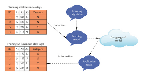
Decision tree is a commonly used classification method in data mining. It predicts and classifies a large number of samples according to certain intentions and hopes to find some information that has reference value for decision-makers. It is a kind of supervised learning; that is, given a bunch of samples, they have a set of attributes and a clear class label in advance by learning these samples to create a classifier so that it can make correct classification judgments for the newly added samples. The classification process generally includes two steps: model construction and prediction application. Taking Figure 3 as an example, the training set has 4 samples of known categories. Through the induction of the training set, a classification model (induction) is established, and the test set is predicted (inference) based on the built model.

Entropy is a common indicator used to measure the purity of sample data. If the uncertainty of the information is greater, the possibility of various situations is greater, and the value of entropy is greater. The mathematical definition is shown in the following formula:

()

Among them, S is the sample set, c is the total number of characteristic attributes, and p is the probability of occurrence of the sample event.

Information gain refers to the change in entropy before and after information division, that is, the expected entropy reduction caused by using a certain attribute A to divide the sample. This is the difference between the original information entropy and the information entropy after the attribute A divides the sample S. The mathematical definition is shown in the following formula:

()

Among them, A is a characteristic attribute, Values(A) is the value range of characteristic attribute A, and Sv is a collection of examples in S whose attribute A is v.

Split Information metric is the number and size information of the branch when a certain attribute is considered for splitting. It is called the intrinsic information of the attribute. The mathematical definition is shown in the following formula:

()

Information gain ratio is the ratio of information gain to intrinsic information. We suppose that the sample set s is divided into c subsets according to c different values of the discrete attributes, and the information gain rate of these subsets is shown in the following formula:

()

Before the nonleaf nodes of the decision tree are split, the information gain rate of each feature attribute is first calculated, and the attribute with the largest information gain rate is selected as the split node. The greater the information gain rate, the stronger the ability to distinguish samples and the more representative it is. This is a top-down greedy strategy. The decision tree model in the article is constructed using the C4.5 algorithm.

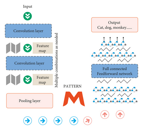
A typical CNN network includes convolution layer, pooling layer, and fully connected layer, and its network structure is shown in Figure 4.

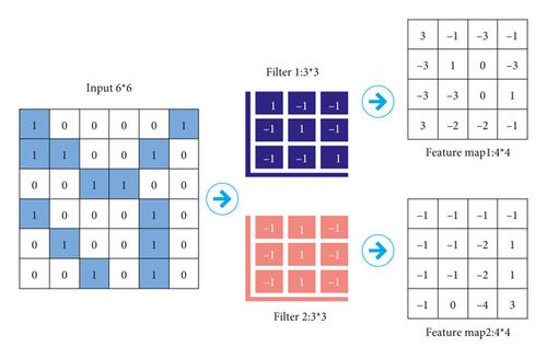
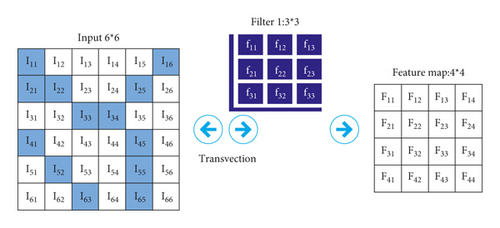
(1) Input Layer ⟶ Convolutional Layer. We assume that the input is a 6 × 6 image and use two 3 × 3 convolution kernels (filter) for convolution, and the stride is set to 1 to obtain two 4 × 4 feature maps, as shown in Figure 5.

The image is input into the CNN, and the feature map is obtained after the convolutional layer. Feature map size calculation method is as follows: [Input size − Filter size]/Stride + 1. Taking Filter 1 as an example, as shown in Figure 6, stride = l, the size of the calculated feature map is 4 × 4, and the F₁₁ input of the first neuron is as follows:

()

The output of the neuron is as follows (using the ReLU activation function):

()

After the convolution operation, the activation function performs a nonlinear transformation on the output of the convolution layer to enhance the expressive ability of the model. It retains and maps the features of activated neurons through the function, which is the key to solving nonlinear problems.

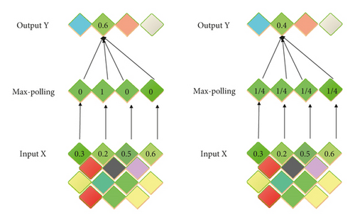
(2) Convolutional Layer ⟶ Pooling Layer. Pooling usually has two forms: mean pooling and max pooling. In essence, they are both a special convolution process, as shown in Figure 7.

In the maximum pooling convolution kernel, only one of the weights is 1, and the rest are 0. The position of 1 in the convolution kernel corresponds to the position where the part of input covered by the convolution kernel has the largest value. The sliding step of the convolution kernel in the original input is 2, which is equivalent to reducing the original input to 1/4 of the original and retaining the strongest input in each 2 × 2 area.

Each weight in the mean pooling convolution kernel is 0.25, and the sliding step of the convolution kernel in the original input is 2, which is equivalent to reducing the original input to 1/4 of the original.

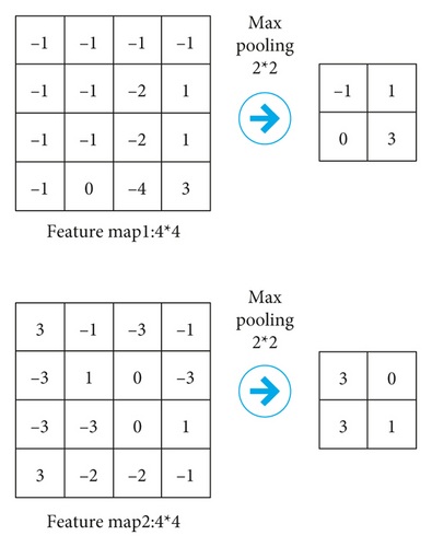
On the basis of Figure 5, it performs a 2 × 2 maximum pooling operation, stride = 2, and the result is shown in Figure 8.

The purpose of the pooling layer is mainly to compress pictures and reduce parameters without affecting the quality of the input image through downsampling. A convolution kernel and a subsampling constitute the unique feature extractor of CNN. Different convolution kernels extract different features. In the two convolution kernel filters in Figure 5, one is responsible for extracting features in the diagonal direction, and the other is responsible for extracting features in the vertical direction. After it executes max pooling, it obtains the value that can really identify the feature, and the rest is discarded. In the subsequent calculation, the size of the feature map is reduced, and the amount of model calculation is reduced.

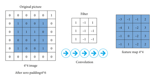
Figure 9 shows a case of zero-padding operation.

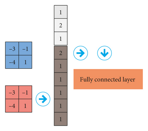
(3) Pooling Layer ⟶ Fully Connected Layer. The output of pooling is sent to the flatten layer to “flatten” all elements as the input of the fully connected layer, as shown in Figure 10.

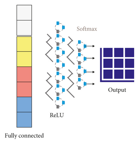
(4) Fully Connected Layer ⟶ Output Layer. The connection method of the fully connected layer to the output layer is the same as that of the traditional neural network. The specific method is to first flatten the output of the pooling layer into a one-dimensional vector, send it to the fully connected layer, and then fully connect with the output layer. Among them, the ReLU function is used as the activation function of the hidden layer, and the SoftMax function is used as the activation function of the output layer. Its purpose is to normalize the output result. For the model classification problem, the input neuron is trained to output the probability value of 1 after the model is trained, as shown in Figure 11.

(1)
Confusion Matrix. We assume that there are only two types of classification targets: positive, represented by 1, and negative, represented by 0. They are the results of the model. Then, there are
True Positives (TP), which is the number of samples that are correctly classified as positive; False Positives (FP), which is the number of samples that are incorrectly classified as positive; False Negatives (FN), which is the number of samples that are incorrectly classified as negative examples; True Negatives (TM), which is the number of samples that are correctly classified as negative examples.
(2)
Evaluation Index.
- ①
  Accuracy is the most common evaluation index, reflecting the overall performance of the model. It can judge positive as positive and negative as negative. Generally speaking, the higher the correct rate, the better the model performance.
  ()
- The opposite of the correct rate is the error rate, which describes the proportion of samples that are misclassified by the model. For instance, correct classification and wrong classification are mutually exclusive; that is, error rate = 1− Accuracy.
- ②
  Precision is a measure of accuracy, which refers to the degree of agreement between the predicted value and the true value, that is, the ratio of the number of correct positive cases to the total number of positive cases predicted.
  ()
- ③
  Recall, also known as “recall rate,” is a measure of coverage, that is, the ratio of the number of positive cases predicted to the number of true positive cases.
  ()
- ④
  F1 score refers to the harmonic mean value of precision rate and recall rate. Generally speaking, the accuracy rate and the recall rate reflect the model performance from two perspectives, and the overall performance of the model cannot be comprehensively measured based on a certain index alone. In order to balance the influence of the two, F1 score is introduced as a comprehensive index to comprehensively evaluate the performance of the model.
  ()
- ⑤
  Sensitivity, also known as True Positive Tate (TPR), is a measure of the model’s ability to discriminate positive examples, which represents the proportion of all positive examples that are correctly classified.
  ()
- False Positive Rate (FPR) is a measure of the proportion of negative cases that the model incorrectly judges as positive; that is, FPR = FP/(FP + TN).
- ⑥
  Specificity, also known as True Negative Rate (TNR), is a measure of the model’s ability to discriminate negative samples, which represents the proportion of all negative cases that are correctly classified.
  ()
- In fact, the sensitivity is the recall rate, and the specificity is 1 FPR.
- ⑦
  Other indicators include the following:

Calculation speed: it is the time spent on model training and prediction.

Robustness: it is the ability of the model to deal with missing values and outliers.

Scalability: it is the ability of the model to handle large datasets.

Interpretability: it is the comprehensibility of the model prediction standard.

4. 3D CAD Classification Model Based on Knowledge Recognition Algorithm of Convolutional Neural Network

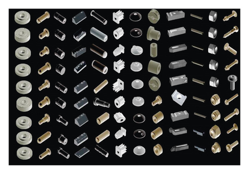
The models in the TracePartsOnline model library are from many manufacturing and processing industries around the world and are created by experienced engineers. The data in the entire database is divided into three parts: training set, label set, and test set, and 1430, 278, and 278 data samples are allocated, respectively. The training set and label set are used to generate the weights and biases of the deep neural network, and the test set is used to evaluate the learning effect. Figure 12 shows a small number of models from the 3D CAD model database.

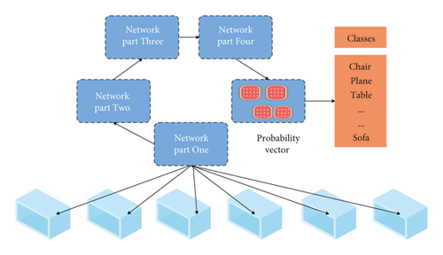
The CNN model consists of 5 convolutional layers (Conv1, Conv2, Conv3, Conv4, and Conv5), 3 maximum pooling layers (MaxPool1, MaxPool2, and MaxPool3), a view pooling layer (ViewPool), and two fully connected layers (Fc6 and Fc7), and a SoftMax classification layer. According to different functions, our CNN model is divided into four parts, as shown in Figure 13.

On the basis of the above model research, the progress of the model proposed in this paper can be verified, the classification effect of the 3D CAD model is counted, and the results are shown in Table 2 and Figure 14.

2. Classification effect of 3D CAD model based on knowledge recognition algorithm of convolutional neural network.

No.	CAD classification effect
1	95.17
2	87.12
3	94.61
4	85.77
5	93.88
6	93.60
7	92.56
8	92.07
9	90.71
10	88.07
11	86.11
12	96.23
13	96.22
14	95.43
15	89.75
16	91.31
17	92.57
18	94.65
19	90.54
20	87.68
21	89.93
22	89.79
23	88.27
24	88.55
25	90.71
26	93.99
27	92.49
28	93.24
29	84.35
30	87.69
31	90.39
32	92.01
33	89.05
34	94.89
35	92.72
36	92.15
37	88.42
38	93.93
39	88.43
40	88.25
41	87.39
42	90.28
43	87.22
44	92.67
45	92.59

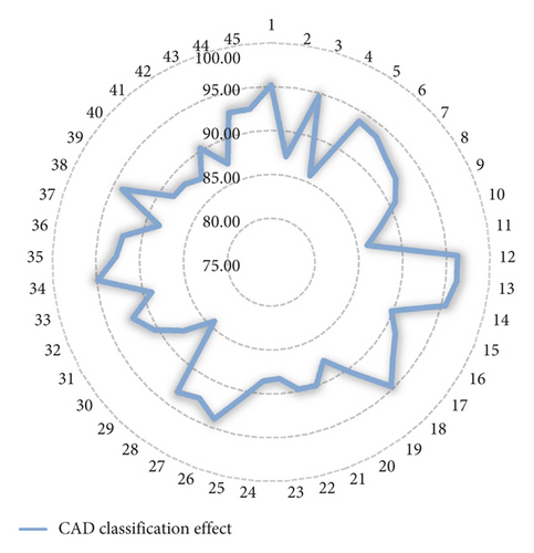
It can be seen from the above research that the 3D CAD classification model based on the knowledge recognition algorithm of convolutional neural network proposed in this paper can play an important role in 3D CAD classification and effectively improve the classification effect of CAD models.

5. Conclusion

Since the classification of industrial CAD models requires a wealth of professional domain knowledge, in most cases, the classification work is mainly carried out by engineers. Traditional automatic classification algorithms extract feature descriptors by designing a certain feature description extraction algorithm by the user and use machine learning algorithms to complete the automatic classification of the model. However, due to the complexity of the 3D model itself, this user-designed feature descriptor extraction algorithm is difficult to completely and accurately capture the feature information of the 3D model, and its expression ability is limited. Shallow machine learning has the disadvantage of restricting the expression effect of functions that are inherently difficult to solve due to insufficient training set and computing power. This paper combines the knowledge recognition algorithm of convolutional neural network to construct the 3D CAD classification model, improve the classification effect of 3D CAD model, and enhance the work efficiency of industrial design. The experimental research results show that the 3D CAD classification model based on the knowledge recognition algorithm of convolutional neural network proposed in this paper can effectively improve the classification effect of the CAD model.

Conflicts of Interest

The authors declare no conflicts of interest.

Open Research

Data Availability

The labeled dataset used to support the findings of this study are available from the corresponding author upon request.

References

1 Poshekhonov R. A., Arutyunyan G. A., Pankratov S. A., Osipkov A. S., Onishchenko D. O., and Leontyev A. I., Development of a mathematical model for optimizing the design of an automotive thermoelectric generator taking into account the influence of its hydraulic resistance on the engine power, Semiconductors. (2017) 51, no. 8, 981–985, https://doi.org/10.1134/s1063782617080255, 2-s2.0-85028353239.
10.1134/S1063782617080255
CAS Web of Science® Google Scholar
2 Uysal F., Phase-coded fmcw automotive radar: system design and interference mitigation, IEEE Transactions on Vehicular Technology. (2019) 69, no. 1, 270–281, https://doi.org/10.1109/tvt.2019.2953305.
10.1109/TVT.2019.2953305
Web of Science® Google Scholar
3 Geren N., Akçalı O. O., and Bayramoğlu M., Parametric design of automotive ball joint based on variable design methodology using knowledge and feature-based computer assisted 3d modelling, Engineering Applications of Artificial Intelligence. (2017) 66, no. nov, 87–103, https://doi.org/10.1016/j.engappai.2017.08.011, 2-s2.0-85030149905.
10.1016/j.engappai.2017.08.011
Web of Science® Google Scholar
4 Mcharek M., Azib T., Hammadi M., Larouci C., and Choley J.-Y., Multiphysical design approach for automotive electronic throttle body, IEEE Transactions on Industrial Electronics. (2020) 67, no. 8, 6752–6761, https://doi.org/10.1109/tie.2019.2939999.
10.1109/TIE.2019.2939999
Web of Science® Google Scholar
5 Xie Y., Zeng G., Kurachi R., Peng X., Xie G., and Takada H., Balancing bandwidth utilization and interrupts: two heuristic algorithms for the optimized design of automotive cps, IEEE Transactions on Industrial Informatics. (2020) 16, no. 4, 2382–2392, https://doi.org/10.1109/tii.2019.2936240.
10.1109/TII.2019.2936240
Web of Science® Google Scholar
6 Trovao J. P., Digital transformation, systemic design, and automotive electronics [automotive electronics], IEEE Vehicular Technology Magazine. (2020) 15, no. 2, 149–159, https://doi.org/10.1109/mvt.2020.2980097.
10.1109/MVT.2020.2980097
Web of Science® Google Scholar
7 Rohde-Brandenburger K. and Koffler C., Commentary on ’correction to: on the calculation of fuel savings through lightweight design in automotive life cycle assessments’ by koffler and rohde-brandeburger (2018), International Journal of Life Cycle Assessment. (2019) 24, no. 3, 397–399, https://doi.org/10.1007/s11367-019-01585-y, 2-s2.0-85060349313.
10.1007/s11367-019-01585-y
Web of Science® Google Scholar
8 Di Pasquale E. and Coutellier D., Wave propagation in head on bonnet impact: material and design issues, International Journal of Automotive Technology. (2017) 18, no. 4, 631–642, https://doi.org/10.1007/s12239-017-0063-z, 2-s2.0-85019727034.
10.1007/s12239-017-0063-z
Web of Science® Google Scholar
9 Nordelöf A., Grunditz E., Tillman A.-M., Thiringer T., and Alatalo M., A scalable life cycle inventory of an electrical automotive traction machine-Part I: design and composition, International Journal of Life Cycle Assessment. (2018) 23, no. 1, 55–69, https://doi.org/10.1007/s11367-017-1308-9, 2-s2.0-85017114201.
10.1007/s11367-017-1308-9
Web of Science® Google Scholar
10 Ayoub H. S., Hussein W. M., El-Sherif A. F., and Elbashar Y. H., Design and test of high-efficiency dual-element laser diffuser for large-field automotive shadowgraphy, Journal of Optics. (2020) 49, no. 2, 263–269, https://doi.org/10.1007/s12596-020-00602-w.
10.1007/s12596-020-00602-w
Web of Science® Google Scholar
11 Kongwat S., Jongpradist P., and Hasegawa H., Lightweight bus body design and optimization for rollover crashworthiness, International Journal of Automotive Technology. (2020) 21, no. 4, 981–991, https://doi.org/10.1007/s12239-020-0093-9.
10.1007/s12239-020-0093-9
Web of Science® Google Scholar
12 Yusof N. S. B., Sapuan S. M., Sultan M. T. H., and Jawaid M., Conceptual design of oil palm fibre reinforced polymer hybrid composite automotive crash box using integrated approach, Journal of Central South University. (2020) 27, no. 1, 64–75, https://doi.org/10.1007/s11771-020-4278-1.
10.1007/s11771-020-4278-1
CAS Web of Science® Google Scholar
13 Hosseini S. M., Arjomandi Rad M., Khalkhali A., and Saranjam M. J., Optimal design of the s-rail family for an automotive platform with novel modifications on the product-family optimization process, Thin-Walled Structures. (2019) 138, no. MAY, 143–154, https://doi.org/10.1016/j.tws.2019.01.046, 2-s2.0-85061354634.
10.1016/j.tws.2019.01.046
Web of Science® Google Scholar
14 Wang T. J. and Hwang S. K., Combustion system design of a genset diesel engine by using dfss methodology, International Journal of Automotive Technology. (2019) 20, no. 3, 539–547, https://doi.org/10.1007/s12239-019-0051-6, 2-s2.0-85066304755.
10.1007/s12239-019-0051-6
Web of Science® Google Scholar
15 Xie G., Peng H., Huang J., Li R., and Li K., Energy-efficient functional safety design methodology using ASIL decomposition for automotive cyber-physical systems, IEEE Transactions on Reliability. (2019) 23, no. 99, 1–23, https://doi.org/10.1109/tr.2019.2915818.
10.1109/tr.2019.2915818
CAS Google Scholar
16 Belgiovane D. J., Chen C. C., Chien Y. P., and Sherony R., Surrogate bicycle design for millimeter-wave automotive radar pre-collision testing, IEEE Transactions on Intelligent Transportation Systems. (2017) 17, no. 9, 1–10, https://doi.org/10.1109/tits.2016.2642889, 2-s2.0-85010689306.
10.1109/tits.2016.2642889
Google Scholar
17 Suh K. and Yoon H., Design optimization of a rear independent suspension for the Korean light tactical vehicle, International Journal of Automotive Technology. (2018) 19, no. 2, 245–252, https://doi.org/10.1007/s12239-018-0023-2, 2-s2.0-85042650152.
10.1007/s12239-018-0023-2
Web of Science® Google Scholar
18 Zhu X., Zheng Y., Qi L., Wang N., and Ni S., Research On Recognition Algorithm Of Tunnel Leakage Based On Image Processing, No. 2020-01-5133, 2020, SAE Technical Paper, New York, NY.
Google Scholar
19 Kong B. S. and Park D. K., Design optimization of the cowl cross bar - light cowl cross bar satisfying 5 performances -, International Journal of Automotive Technology. (2018) 19, no. 3, 387–391, https://doi.org/10.1007/s12239-018-0037-9, 2-s2.0-85044989559.
10.1007/s12239-018-0037-9
Web of Science® Google Scholar
20 Cai Y., Ouyang M., and Yang F., Energy management and design optimization for a series-parallel phev city bus, International Journal of Automotive Technology. (2017) 18, no. 3, 473–487, https://doi.org/10.1007/s12239-017-0047-z, 2-s2.0-85016808674.
10.1007/s12239-017-0047-z
Web of Science® Google Scholar
21 Zhang R., Li K., Yu F., He Z., and Yu Z., Novel electronic braking system design for evs based on constrained nonlinear hierarchical control, International Journal of Automotive Technology. (2017) 18, no. 4, 707–718, https://doi.org/10.1007/s12239-017-0070-0, 2-s2.0-85019750043.
10.1007/s12239-017-0070-0
Web of Science® Google Scholar

All articles

Classification of 3D CAD Models considering the Knowledge Recognition Algorithm of Convolutional Neural Network

Abstract

1. Introduction

2. Related Work

3. Knowledge Recognition of the Convolutional Neural Network

3.1. Synthesis Rules

3.2. Decision Rules

3.2.1. The LVQ1 Algorithm

3.2.2. The LVQ2 Algorithm

4. 3D CAD Classification Model Based on Knowledge Recognition Algorithm of Convolutional Neural Network

5. Conclusion

Conflicts of Interest

Open Research

Data Availability

References

Figures

References

Information

About Wiley Online Library

Help & Support

Opportunities

Connect with Wiley