Volume 2022, Issue 1 1713912

Research Article

Open Access

The Construction and Approximation of ReLU Neural Network Operators

Hengjie Chen

orcid.org/0000-0002-9143-9945

Department of Mathematical Sciences, School of Science, Zhejiang Sci-Tech University, Hangzhou 310018, China zstu.edu.cn

Search for more papers by this author

Dansheng Yu,

Dansheng Yu

orcid.org/0000-0003-3378-3251

School of Mathematics, Hangzhou Normal University, Hangzhou 310036, China hznu.edu.cn

Search for more papers by this author

Zhong Li,

Corresponding Author

Zhong Li

[email protected]

orcid.org/0000-0002-2730-6427

Department of Mathematical Sciences, School of Science, Zhejiang Sci-Tech University, Hangzhou 310018, China zstu.edu.cn

School of Information Engineering, Huzhou University, Huzhou 313000, China zjhu.edu.cn

Search for more papers by this author

Hengjie Chen,

Hengjie Chen

orcid.org/0000-0002-9143-9945

Department of Mathematical Sciences, School of Science, Zhejiang Sci-Tech University, Hangzhou 310018, China zstu.edu.cn

Search for more papers by this author

Dansheng Yu,

Dansheng Yu

orcid.org/0000-0003-3378-3251

School of Mathematics, Hangzhou Normal University, Hangzhou 310036, China hznu.edu.cn

Search for more papers by this author

Zhong Li,

Corresponding Author

Zhong Li

[email protected]

orcid.org/0000-0002-2730-6427

Department of Mathematical Sciences, School of Science, Zhejiang Sci-Tech University, Hangzhou 310018, China zstu.edu.cn

School of Information Engineering, Huzhou University, Huzhou 313000, China zjhu.edu.cn

Search for more papers by this author

First published: 28 September 2022

https://doi.org/10.1155/2022/1713912

Citations: 2

Academic Editor: Yoshihiro Sawano

Share a link

Email
Wechat
Bluesky

Abstract

In the present paper, we construct a new type of two-hidden-layer feedforward neural network operators with ReLU activation function. We estimate the rate of approximation by the new operators by using the modulus of continuity of the target function. Furthermore, we analyze features such as parameter sharing and local connectivity in this kind of network structure.

1. Introduction

Artificial neural network is a fundamental method in machine learning, which has been applied in many fields such as pattern recognition, automatic control, signal processing, auxiliary decision-making, and artificial intelligence. In particular, the successful applications of deep (multihidden layer) neural networks in image recognition, natural language processing, computer vision, etc. developed in recent years have made neural networks attract great attention. In fact, ever the function of XOR gate was implemented by adding one layer from the simplest perceptron, which leaded to the single-hidden-layer feedforward neural network.

A single-hidden-layer feedforward neural network has the expression form

(1)

where c_i, θ_i(i = 1, 2, ⋯, n) are called as output weights and thresholds, the dimension of input weights ω_i(i = 1, 2, ⋯, n) corresponds to that of the input x, ϕ, is called the activation function of this network, and n₁ is the number of neurons in the hidden layer. If

(T denotes the transpose) is the input weight matrix of size

and

are vectors of thresholds and output weights, respectively, then (1) can be written as

(2)

where ϕ(A₁x + Θ₁) means that ϕ acts on each component of A₁x + Θ₁. Now, the architecture of the neural network with two hidden layers is really not difficult to understand. If the second hidden layer contains n₂ neurons, the input weight matrix A₂ is the size of n₂ × n₁, the vector of thresholds is Θ₂, and the output weight vector is O; then, the two-hidden-layer feedforward neural network can be mathematically expressed as

(3)

We call w = max{n₁, n₂} as the width of the network , and its depth is naturally 2.

The theoretical research and applications of the single-hidden-layer neural network model had been greatly developed in the 80’s and 90’s of last century; particularly, there were also some research results on the neural networks with multihidden layers at that time. So, in [1], Pinkus pointed out that “Nonetheless there seems to be reasonable to conjecture that the two-hidden-layer model may be significantly more promising than the single layer model, at least from a purely approximation-theoretical point of view. This problem certainly warrants further study.” However, whether it is a single-hidden-layer or multihidden-layer neural network, three fundamental issues are always involved: density, complexity, and algorithms.

The so-called density or universal approximation of a neural network structure means that for any given error accuracy and the target function in a function space with some metrics, there is a specific neural network model (except for the input x, other parameters are determined) such that the error between the output and target is less than the preaccuracy. In the 1980s and 1990s, the research on the density of feedforward neural network has achieved many satisfactory results [2–9]. Since the single-hidden-layer neural network is an extreme case of the multilayer neural networks, the current focus of neural network research is still on complexity and algorithms. So-called the complexity of a neural network means that to guarantee a prescribed degree of approximation, a neural network model requires the numbers of structural parameters, including the number of layers (or depth), the number of neuron in each layer (sometimes use width), and the number of link weights and the number of thresholds. In particular, it is of interest to have more equal weights and thresholds, which is called as the parameter sharing, as this reduces computational complexity. The representation ability that has attracted much attention in deep neural networks is actually the study of complexity problem, which needs to be investigated extensively and urgently.

The constructive method is an important approach to the study of complexity, which is applicable to single- and multiple-hidden-layer neural network. In fact, there are two cases here: one is that the depth, width, and approximation degree are given, while the weights and thresholds are uncertain; the other is that all these are given; that is, the neural network model is completely determined. In order to determine the weights and thresholds in the first kind of neural network, we simply use samples to learn or train. Theoretically, the second kind of neural network can be applied directly, but the parameters are often fine-tuned with a small number of samples before use. There have been many results about the constructions of network operators [10–26]. It can be seen that these research results have an important guiding role in the construction and design of neural networks. Therefore, the purpose of this paper is to construct a kind of two-hidden-layer feedforward neural network operators with the ReLU activation function, and the upper bound estimate of approximation (or regression) ability of this neural network for two variable continuous function defined on [−1, 1]² is given.

The rest of the paper is organized as follows: in Section 2, we introduce new two-hidden-layer neural network operators with ReLU activation function and give the approximation rate of approximation by the new operators. In Section 3, we give the proof of the main result. Finally, in Section 4, we give some numerical experiments and discussions.

2. Construction of ReLU Neural Network Operators and Its Approximation Properties

Let r : ℝ⟶ℝ denote the rectified linear unit (ReLU), i.e., r(x) = max{0, x}. For any (x₁, x₂) ∈ ℝ × ℝ≕ℝ², we define

(4)

Obviously, σ is a continuous function of two variables supported on [−1, 1]². By using the fact that |x| = r(x) + r(−x), σ can be rewritten as follows:

(5)

From the above representation, we see that σ(x₁, x₂) can be explained as the output of a two-hidden-layer feedforward neural network. It is obvious that σ possesses the following some important properties:

(A1) σ(−x₁, x₂) = σ(x₁, x₂), σ(x₁, −x₂) = σ(x₁, x₂)

(A2) For any given x₁ ∈ ℝ, σ(x₁, x₂), it is nondecreasing for x₂ ≤ 0 and nonincreasing for x₂ ≥ 0. Simultaneously, for any given x₂ ∈ ℝ, σ(x₁, x₂),it is nondecreasing for x₁ ≤ 0 and nonincreasing for x₁ ≥ 0

(A3) 0 ≤ σ(x₁, x₂) ≤ 3/4

(A4)

For any continuous function f(x₁, x₂) on [−1, 1]², we define the following neural network operator:

(6)

where ⌊x⌋ is the largest integer not greater than x, and ⌈x⌉ denotes the smallest integer not less than x.

We prove that the rate of approximation by can be estimated by using the modulus of smoothness of the target function. In fact, we have

Theorem 1. Let f(x₁, x₂) is a continuous function defined on [−1, 1]². Then,

(7)

where and are the modulus of continuity of f defined by

(8)

Remark 2. For 0 < α < 1, we define the following neural network operators:

(9)

Using a similar process of the proof in Theorem 1, we can get

(10)

Remark 3. Let β (0 < β ≤ 1) be a fixed number, if there is a constant L > 0 such that

(11)

for any (x₁, x₂), (x_1′, x_2′) ∈ [−1, 1]², we say that f is a Lipschitz function of order β and write

. Obviously, when

, we have

. Consequently, it follows from (7) that

(12)

Remark 4. Now, we describe the structure of by using the form (3).

The input matrix of the first hidden layer is

(13)

and its size is . The bias vector of the first hidden layer is

(14)

and the dimension is . The input matrix of the second hidden layer is

(15)

and its size is . Θ₂ is a constant 1 vector with dimension . The output weight vector is

(16)

Its general term and dimension are

and

, respectively.

We can see that there are two different numbers in weight matrices A₁ and A₂, respectively. That is, neural network operators have a strong weight sharing feature. There are some results about the constructions of this kind of neural networks [14, 27–29]. Moreover, A₂ shows that this neural network is locally connected. Finally, the simplicity of bias vector Θ₂ also greatly reduces the complexity of the neural network.

3. Proof of the Main Result

To prove Theorem 1, we need the following auxiliary lemma.

Lemma 5. For function σ(x₁, x₂), we have

(17)

Proof. We only prove (1), and (2), (3), and (4) can be proved similarly.

(1)
When k_i − 1 < k_i < k_i + 1 ≤ [nx_i] − 1(i = 1, 2), we have

(18)

Considering the monotonicity of σ(x₁, x₂), we have

(19)

(20)

Combining (19) and (20) leads to

(21)

Similarly, we have

(22)

By (21), (22), and summation from to [nx_i] − 1(i = 1, 2), we obtain (1) of Lemma 5.

(2)
When k₂ + 1 > k₂ > k₂ − 1 ≥ ⌈nx₂⌉ + 1, we have

(23)

From (18), (23), and in a similar way to the proof in proving (1), we get

(24)

By summation for and , we obtain (2) of Lemma 5.

Proof of Theorem 6. Let

(25)

Then,

(26)

We further estimate by estimating I₁ and I₂, respectively.

Set

(27)

Since in ∑² + ∑³ + ∑⁴, at least one of inequalities and holds; so, either

(28)

(29)

is valid. Therefore,

(30)

which implies that

(31)

For ∑¹, by the facts that , for (x₁, x₂) ∈ [−1, 1]², we obtain that

(32)

Hence,

(33)

where we have used the inequality 0 ≤ σ ≤ 3/4, and the fact that the number of the terms in ∑¹ is no more than . From (27)-(33), it follows that

(34)

Set

(35)

Then,

(36)

Firstly, we have

(37)

Noting that , we get Δ₁ = 0 by the similar arguments for estimating ∑² + ∑³ + ∑⁴ in (27). Therefore,

(38)

Consequently,

(39)

Similarly, we have

(40)

Thus, we already have

(41)

Now, let us estimate I₂₁. By

(42)

we deduce that

(43)

where we used the fact that the support of σ(t₁, t₂) is [−1, 1]².

Similarly, by

(44)

we have

(45)

By (1) of Lemma 5, (43), and (45), we have

(46)

By (2)-(4) of Lemma 5, and the arguments similar to (43) and (45), we obtain that

(47)

(48)

(49)

By (46)-(49) and the identity , we have

(50)

It follows from (26), (34)-(41), and (50) that

(51)

which completes the proof of Theorem 6.

4. Numerical Experiments and Some Discussions

In this section, we give some numerical experiments to illustrate the theoretical results. We take as the target function.

Set

(52)

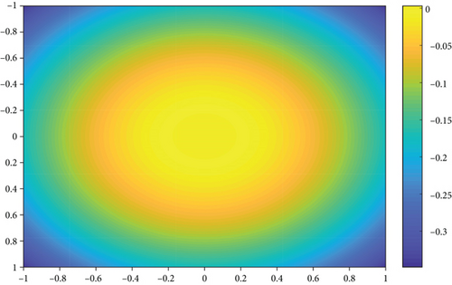
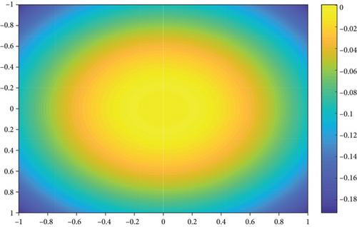
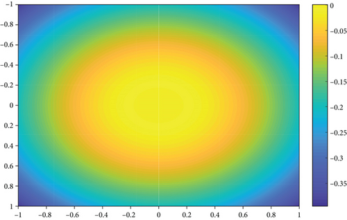
Figures 1–3 show the results of e₁₀₀(x₁, x₂), e₁₀₀₀(x₁, x₂) and e₁₀₀₀₀(x₁, x₂), respectively. When n equals to 10⁶, the amount of calculation of is large. Therefore, we choose 6 specific points and the corresponding values of e_n(x₁, x₂), which are shown in Table 1.

Details are in the caption following the image — **Figure 1**
Open in figure viewer PowerPoint

Errors of approximation of network operators (6) with n = 100.

Table 1. The error values of e_n(x₁, x₂) for 6 specific points with n = 1000000.

(x₁, x₂)	(0, −1)	(−1, 1)	(0.5,0.5)	(0, 0)	(0.5, −0.6)	(0.25,0.8)
e_n(x₁, x₂)	0.0020	0.0040	-9.982e-04	3.992e-07	0.0012	-0.0014

From the results of experiments we see that as the parameter n of neural network operators increases, the approximation effect increases; we only need to notice , and after the simple calculation, we can demonstrate the validity of the obtained result.

If we investigate network operators (6) carefully, we cannot help but ask why we use

instead of f((k₁/n), (k₂/n)) in (6). Because ((k₁/n), (k₂/n)) are the conventional grid points on [−1, 1]², this will reduce the amount of calculation. Now, we might as well introduce the following network operators:

(53)

Then, from the proof of Theorem 6, we have

(54)

It is not difficult to obtain the same estimate of I^′ as I₁, but it is not inconvenient to estimate

. In fact, if we set

(55)

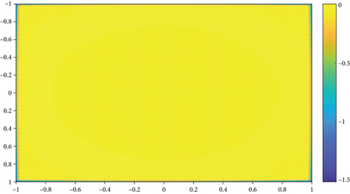
Figure 4 shows the with n = 1000. We can see that next to the border of [−1, 1]² the effect of approximating f is not satisfactory. Particularly, we can see this phenomenon from Table 2 below. So, we modified f((k₁/n), (k₂/n)) to construct operators (6). Then, we obtain the error estimation of approximation of operators (6) and give the numerical experiments.

Table 2. The error values of

and e_n(x₁, x₂) for 6 specific points with n = 10000.

(x₁, x₂)	(0, −1)	(−1, 1)	(0.5,0.5)	(0, 0)	(0.5, −0.6)	(0.25,0.8)
	-0.5000	-1.4862	2.749e-05	3.999e-05	2.47e-05	2.24e-05
e_n(x₁, x₂)	-0.0197	-0.0394	-0.0098	3.921e-05	-0.0120	-0.0138

Conflicts of Interest

The authors declare that they have no conflicts of interest.

Acknowledgments

This research was supported by the National Natural Science Foundation of China under Grant No. 12171434 and Zhejiang Provincial Natural Science Foundation of China under Grant No. LZ19A010002.

Open Research

Data Availability

Data are available on request from the authors.

References

1 Pinkus A., Approximation theory of the MLP model in neural networks, Acta Numerica. (1999) 8, 143–195, https://doi.org/10.1017/S0962492900002919, 2-s2.0-85011438572.
10.1017/S0962492900002919
Google Scholar
2 Chen T. P., Chen H., and Liu R. W., Approximation capability in C(Rⁿ) by multilayer feedforward networks and related problems, IEEE Transactions on Neural Networks. (1995) 6, no. 1, 25–30, https://doi.org/10.1109/72.363453, 2-s2.0-0029207175.
10.1109/72.363453
CAS PubMed Web of Science® Google Scholar
3 Chen T. P. and Chen H., Universal approximation to nonlinear operators by neural networks with arbitrary activation functions and its application to dynamical systems, IEEE Transactions on Neural Networks. (1995) 6, no. 4, 911–917, https://doi.org/10.1109/72.392253, 2-s2.0-0029343809, 18263379.
10.1109/72.392253
CAS PubMed Web of Science® Google Scholar
4 Chui C. K. and Li X., Approximation by ridge functions and neural networks with one hidden layer, Journal of Approximation Theory. (1992) 70, no. 2, 131–141, https://doi.org/10.1016/0021-9045(92)90081-X, 2-s2.0-0000378922.
10.1016/0021-9045(92)90081-X
Web of Science® Google Scholar
5 Cybenko G., Approximation by superpositions of a sigmoidal function, Math. of Control Signals and System. (1989) 2, no. 4, 303–314, https://doi.org/10.1007/BF02551274, 2-s2.0-0024861871.
10.1007/BF02551274
Google Scholar
6 Funahashi K. I., On the approximate realization of continuous mappings by neural networks, Neural Networks. (1989) 2, no. 3, 183–192, https://doi.org/10.1016/0893-6080(89)90003-8, 2-s2.0-0024866495.
10.1016/0893-6080(89)90003-8
Web of Science® Google Scholar
7 Hornik K., Stinchombe M., and White H., Multilayer feedforward networks are universal approximators, Neural Networks. (1989) 2, no. 5, 359–366, https://doi.org/10.1016/0893-6080(89)90020-8, 2-s2.0-0024880831.
10.1016/0893-6080(89)90020-8
Web of Science® Google Scholar
8 Kuková V., Kolmogorov's theorem and multilayer neural networks, Neural Networks. (1992) 5, no. 3, 501–506, https://doi.org/10.1016/0893-6080(92)90012-8, 2-s2.0-0026627415.
10.1016/0893-6080(92)90012-8
Web of Science® Google Scholar
9 Leshno M., Lin V. Y., Pinkus A., and Schocken S., Multilayer feedforward networks with a nonpolynomial activation function can approximate any function, Neural Networks. (1993) 6, no. 6, 861–867, https://doi.org/10.1016/S0893-6080(05)80131-5, 2-s2.0-0027262895.
10.1016/S0893-6080(05)80131-5
Web of Science® Google Scholar
10 Anastassiou G. A., Rate of convergence of some neural network operators to the unit-univariate case, Journal of Mathematical Analysis and Applications. (1997) 212, no. 1, 237–262, https://doi.org/10.1006/jmaa.1997.5494, 2-s2.0-0031195377.
10.1006/jmaa.1997.5494
Web of Science® Google Scholar
11 Anastassiou G. A., Univariate hyperbolic tangent neural network approximation, Mathematical and Computer Modelling. (2011) 53, no. 5-6, 1111–1132, https://doi.org/10.1016/j.mcm.2010.11.072, 2-s2.0-78751604033.
10.1016/j.mcm.2010.11.072
Google Scholar
12 Barron A. R., Universal approximation bounds for superpositions of a sigmoidal function, IEEE Transactions on Information Theory. (1993) 39, no. 3, 930–945, https://doi.org/10.1109/18.256500, 2-s2.0-0027599793.
10.1109/18.256500
Web of Science® Google Scholar
13 Cao F., Xie T., and Xu Z. B., The estimate for approximation error of neural networks: a constructive approach, Neurocomputing. (2008) 71, no. 4-6, 626–630, https://doi.org/10.1016/j.neucom.2007.07.024, 2-s2.0-38649094938.
10.1016/j.neucom.2007.07.024
Web of Science® Google Scholar
14 Cao F. and Xie T., The construction and approximation for feedforword neural networks with fixed weights, 2010 International Conference on Machine Learning and Cybernetics, 2010, Qingdao, China, 3164–3168, https://doi.org/10.1109/ICMLC.2010.5580706, 2-s2.0-78149319498.
10.1109/ICMLC.2010.5580706
Google Scholar
15 Chen D. B., Degree of approximation by superpositions of a sigmoidal function, Approximation Theory and its Applications. (1993) 9, 17–28.
10.1007/BF02836480
Google Scholar
16 Chen Z. and Cao F., The approximation operators with sigmoidal functions, Computers & Mathematics with Applications. (2009) 58, no. 4, 758–765, https://doi.org/10.1016/j.camwa.2009.05.001, 2-s2.0-67649743440.
10.1016/j.camwa.2009.05.001
Web of Science® Google Scholar
17 Chen L. and Wu C. W., A note on the expressive power of deep rectified linear unit networks in high- dimensional spaces, Mathematicsl Methods in the Applied Sciences. (2019) 42, no. 9, 3400–3404, https://doi.org/10.1002/mma.5575, 2-s2.0-85065243241.
10.1002/mma.5575
Web of Science® Google Scholar
18 Costarelli D., Interpolation by neural network operators activated by ramp functions, Journal of Mathematical Analysis and Applications. (2014) 419, no. 1, 574–582, https://doi.org/10.1016/j.jmaa.2014.05.013, 2-s2.0-84902360925.
10.1016/j.jmaa.2014.05.013
Web of Science® Google Scholar
19 Costarelli D., Neural network operators: constructive interpolation of multivariate functions, Neural Networks. (2015) 67, 28–36, https://doi.org/10.1016/j.neunet.2015.02.002, 2-s2.0-84926293410, 25864121.
10.1016/j.neunet.2015.02.002
PubMed Web of Science® Google Scholar
20 Costarelli D. and Vinti G., Voronovskaja type theorems and high-order convergence neural network operators with sigmoidal functions, Mediterranean Journal of Mathematics. (2020) 17, no. 3, https://doi.org/10.1007/s00009-020-01513-7.
10.1007/s00009-020-01513-7
Web of Science® Google Scholar
21 Daubechies I., Devore R., Foucart S., Hanin B., and Petrova G., Nonlinear approximation and (deep) ReLU networks, Constructive Approximation. (2022) 55, no. 1, 127–172, https://doi.org/10.1007/s00365-021-09548-z.
10.1007/s00365-021-09548-z
Web of Science® Google Scholar
22 Mhaskar H. N. and Micchelli C. A., Degree of approximation by neural and translation networks with a single hidden layer, Advances in Applied Mathematics. (1995) 16, no. 2, 151–183, https://doi.org/10.1006/aama.1995.1008, 2-s2.0-0000194429.
10.1006/aama.1995.1008
Web of Science® Google Scholar
23 Qian Y. Y. and Yu D. S., Rates of approximation by neural network interpolation operators, Applied Mathematics and Computation. (2022) 418, article 126781, https://doi.org/10.1016/j.amc.2021.126781.
10.1016/j.amc.2021.126781
Web of Science® Google Scholar
24 Shaham U., Cloninger A., and Coifman R., Provable approximation properties for deep neural networks, Applied and Computational Harmonic Analysis. (2018) 44, no. 3, 537–557, https://doi.org/10.1016/j.acha.2016.04.003, 2-s2.0-84964515172.
10.1016/j.acha.2016.04.003
Web of Science® Google Scholar
25 Yarotsky D., Error bounds for approximations with deep ReLU networks, Neural Networks. (2017) 94, 103–114, https://doi.org/10.1016/j.neunet.2017.07.002, 2-s2.0-85026205840.
10.1016/j.neunet.2017.07.002
PubMed Web of Science® Google Scholar
26 Zhou D. X., Universality of deep convolutional neural networks, Applied and Computational Harmonic Analysis. (2020) 48, no. 2, 787–794, https://doi.org/10.1016/j.acha.2019.06.004.
10.1016/j.acha.2019.06.004
Web of Science® Google Scholar
27 Guliyev N. J. and Ismailov V. E., Approximation capability of two hidden layer feedforward neural networks with fixed weights, Neurocomputing. (2018) 316, 262–269, https://doi.org/10.1016/j.neucom.2018.07.075, 2-s2.0-85052077048.
10.1016/j.neucom.2018.07.075
Web of Science® Google Scholar
28 Guliyev N. J. and Ismailov V. E., On the approximation by single hidden layer feedforward neural networks with fixed weights, Neural Networks. (2018) 98, 296–304, https://doi.org/10.1016/j.neunet.2017.12.007, 2-s2.0-85039766256, 29301110.
10.1016/j.neunet.2017.12.007
PubMed Web of Science® Google Scholar
29 Hahm N. and Hong B. I., An approximation by neural networkswith a fixed weight, Computers & Mathematcs with Applications. (2004) 47, no. 12, 1897–1903, https://doi.org/10.1016/j.camwa.2003.06.008, 2-s2.0-9644287964.
10.1016/j.camwa.2003.06.008
Web of Science® Google Scholar

Citing Literature

All articles

The Construction and Approximation of ReLU Neural Network Operators

Abstract

1. Introduction

2. Construction of ReLU Neural Network Operators and Its Approximation Properties

3. Proof of the Main Result

4. Numerical Experiments and Some Discussions

Conflicts of Interest

Acknowledgments

Open Research

Data Availability

References

Citing Literature

Figures

References

Information

About Wiley Online Library

Help & Support

Opportunities

Connect with Wiley

The Construction and Approximation of ReLU Neural Network Operators

Abstract

1. Introduction

2. Construction of ReLU Neural Network Operators and Its Approximation Properties

3. Proof of the Main Result

4. Numerical Experiments and Some Discussions

Conflicts of Interest

Acknowledgments

Open Research

Data Availability

References

Citing Literature

Figures

References

Related

Information