Convergence Theorems for the Variational Inequality Problems and Split Feasibility Problems in Hilbert Spaces
Abstract
In this paper, we establish an iterative algorithm by combining Yamada’s hybrid steepest descent method and Wang’s algorithm for finding the common solutions of variational inequality problems and split feasibility problems. The strong convergence of the sequence generated by our suggested iterative algorithm to such a common solution is proved in the setting of Hilbert spaces under some suitable assumptions imposed on the parameters. Moreover, we propose iterative algorithms for finding the common solutions of variational inequality problems and multiple-sets split feasibility problems. Finally, we also give numerical examples for illustrating our algorithms.
1. Introduction
Denote by Γ the set of solutions of SFP (2).
Moreover, it is well known that if F is k-Lipschitz continuous and η-strongly monotone, then VIP (4) has a unique solution (see, e.g., [14]).
-
(C1) tn ∈ (0,1), tn⟶0 as n⟶∞ and .
-
(C2) 0 < liminfn⟶∞αn ≤ limsupn⟶∞αn < 1.
Motivated by the aforementioned works, we establish an iterative algorithm by combining algorithms (7) and (8) for finding the solution of problem (6) and prove the strong convergence of the sequence generated by our iterative algorithm to the solution of problem (6) in the setting of Hilbert spaces. Moreover, we propose iterative algorithms for solving the common solutions of variational inequality problems and multiple-sets split feasibility problems. Finally, we also give numerical examples for illustrating our algorithms.
2. Preliminaries
In order to solve our results, we now recall the following definitions and preliminary results that will be used in the sequel. Throughout this section, let C be a nonempty closed convex subset of a real Hilbert space H with inner product 〈⋅, ⋅〉 and norm ‖⋅‖.
Definition 1. A mapping T : H⟶H is called
- (i)
k-Lipschitz continuous, if ‖Tx − Ty‖ ≤ k‖x − y‖ for all x, y ∈ H, where k is a positive number.
- (ii)
Nonexpansive, if (i) holds with k = 1.
- (iii)
η-strongly monotone, if η‖x − y‖2 ≤ 〈Tx − Ty, x − y〉 for all x, y ∈ H, where η is a positive number.
- (iv)
Firmly nonexpansive, if ‖Tx − Ty‖2 ≤ 〈Tx − Ty, x − y〉 for all x, y ∈ H.
- (v)
α-Averaged, if T = (1 − α)I + αN for some fixed α ∈ (0,1) and a nonexpansive mapping N.
In [5], we know that the metric projection PC : H⟶C is firmly nonexpansive and (1/2)-averaged.
We collect some basic properties of averaged mappings in the following results.
Lemma 1 (see [16].)We have
- (i)
The composite of finitely many averaged mappings is averaged. In particular, if Ti is αi-averaged, where αi ∈ (0,1) for i = 1,2, then the composite T1T2 is α-averaged, where α = α1 + α2 − α1α2.
- (ii)
If the mappings are averaged and have a common fixed point, then
Proposition 1 (see [19].)Let D be a nonempty subset of H, m ≥ 2 be an integer, and ϕ; (0,1)m⟶(0,1) be defined by
For every i ∈ {1, …, m}, let αi ∈ (0,1) and Ti : D⟶D be αi-averaged. Then, T = T1, …, Tm is α-averaged, where α = ϕ(α1, …, αm).
The following properties of the nonexpansive mappings are very convenient and helpful to use.
Lemma 2 (see [20].)Assume that H1 and H2 are Hilbert spaces. Let A : H1⟶H2 be a linear bounded mapping such that A ≠ 0 and let T : H2⟶H2 be a nonexpansive mapping. Then, for 0 ≤ γ < 1/‖A‖2, I − γA∗(I − T)A is γ‖A‖2-averaged.
Proposition 2 (see [19].)Let C be a nonempty subset of H, and let be a finite family of nonexpansive mappings from C to H. Assume that and such that ∑i∈Iδi = 1. Suppose that, for every i ∈ I, Ti is -averaged; then, T = ∑i∈IδiTi is α-averaged, where .
The following results play a crucial role in the next section.
Lemma 3 (see [14].)Let t be a real number in (0,1]. Let F : H⟶H be an η-strongly monotone and k-Lipschitz continuous mapping. The mapping I − tμF, for each fixed point μ ∈ (0, (2η/k2)), is contractive with constant 1 − tτ, i.e.,
Theorem 1 (see [21].)Let F be a k-Lipschitz continuous and η-strongly monotone self-mapping of H. Assume that is a finite family of nonexpansive mappings from H to H such that . Then, the sequence {xn} defined by the following algorithm converges strongly to the unique solution x∗ of the variational inequality (4):
- (i)
tn ∈ (0,1), tn⟶0 as n⟶∞ and .
- (ii)
, for some α, β ∈ (0,1), and as n⟶∞, (i = 0, …, N).
3. Main Results
Throughout our results, unless otherwise stated, we assume that H1 and H2 are two real Hilbert spaces and A : H1⟶H2 is a linear bounded mapping. Let F be an η-strongly monotone and k-Lipschitz continuous mapping on H1 with some positive constants η and k. Assume that μ ∈ (0, 2η/k2) is a fixed number.
Theorem 3. Let C and Q be two closed convex subsets in H1 and H2, respectively. Then, as n⟶∞, the sequence {xn} defined by (15), where the sequences {tn} and {αn} satisfy conditions (C1) and (C2), respectively, converges strongly to the solution of (6).
Proof. From Lemma 2, we have that I − γA∗(I − PQ)A is γ‖A‖2-averaged. Since T = PC(I − γA∗(I − PQ)A), by Lemma 1 (i), we get that T is λ-averaged where λ = (1 + γ‖A‖2/2). Moreover, we obtain that z ∈ Γ if and only if z ∈ Fix(T). It follows from Definition 1 (iv) that T = (1 − λ)I + λS, where S is nonexpansive. Then, iterative algorithm (15) can be rewritten as follows:
In [23], Miao and Li showed the weak convergence results of the sequence {xn} converging to the element of Fix(T) where {xn} is generated by the following algorithm:
Theorem 4. Let C and Q be two closed convex subsets in H1 and H2, respectively. Then, as n⟶∞, the sequence {xn} defined by (17), where the sequence {tn} satisfies condition (C1) and {βn} and {αn} satisfy condition (C2), converges strongly to the solution of (6).
Proof. In the proof of Theorem 3, one can rewrite iterative algorithm (17) as follows:
Moreover, we obtain the following results which are solving the common solution of variational inequality problem and multiple-sets split feasibility problem, i.e., find a point
Theorem 5. Let and be two finite families of closed convex subsets in H1 and H2, respectively. Assume that γ ∈ (0, 1/‖A‖2), {tn} and {αn} satisfy conditions (C1) and (C2), respectively, and the parameters {δn} and {ζn} satisfy the following conditions:
- (a)
δi > 0 for 1 ≤ i ≤ N such that .
- (b)
ζj > 0 for 1 ≤ j ≤ M such that .
-
(A1) and
-
(A2) and
-
(A3) and
-
(A4) and ,
Proof. Let T = P1(I − γA∗(I − P2)A). We will show that T is averaged.
In the case of (A1), and . Since is (1/2)-averaged for all i = 1, …, N, by Proposition 1, we get that P1 is λ1-averaged, where λ1 = N/(N + 1). Similarly, we have that P2 is also averaged and so P2 is nonexpansive. By using Lemma 2, we deduce that I − γA∗(I − P2)A is λ2-averaged, where λ2 = γ‖A‖2. It follows from Lemma 1 (i) that T is λ-averaged with λ = N/(N + 1) + γ‖A‖2 − (N/(N + 1))γ‖A‖2.
If and , then by using Proposition 2 and condition (a), we obtain that P1 is (1/2)-averaged. From condition (b) and taking into account that is nonexpansive, for all j = 1, …, M, we have that P2 is also nonexpansive. It follows from Lemma 2 that I − γA∗(I − P2)A is γ‖A‖2-averaged. Thus, T is λ-averaged with λ = (1 + γ‖A‖2)/2.
Cases (A3) and (A4) are similar. This implies that T : = (1 − λ)I + λS, where S is nonexpansive. Moreover, by Lemma 1, we get that
Then, iterative algorithm (20) can be rewritten as follows:
Theorem 6. Let , , and {ζn} be as in Theorem 5. Then, as n⟶∞, the sequence {xn}, defined by
4. Numerical Example
Example 1. We consider test problem (25), where N = M = 1, n = m = 2, φ(x) = (1 − a)‖x‖2/2 for some fixed a ∈ (0,1), and
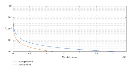
So, we have that F : = φ′ = (1 − a)I is a k-Lipschitz continuous and η-strongly monotone mapping with k = η = (1 − a). For each algorithm, we set ai = (1/i, −1), bi = 0, for all i = 1, …, N, and aj = (1/j, 0), Rj = 1, for all j = 1, …, M. Taking a = 0.5, γ = 0.3, the stopping criterion is defined by En = ‖xn+1 − xn‖ < ε where ε = 10−4 and 10−6. The numerical results are listed in Table 1 with different initial points x1, where n is the number of iterations and s is the CPU time in seconds. In Figures 1 and 2, we present the graphs illustrating the number of iterations for both methods using the stopping criterion defined as above with the different initial points shown in Table 1.
| 10−4 | 10−6 | ||||
|---|---|---|---|---|---|
| Initial point | n | s | n | s | |
| (−2,1)T | Buong method | 29461 | 0.364595 | 2946204 | 31.362283 |
| New method | 11784 | 0.241371 | 1178481 | 23.411679 | |
| (1,3)T | Buong method | 30632 | 0.565431 | 3063343 | 33.468210 |
| New method | 12252 | 0.324808 | 1225336 | 25.570356 | |


Remark 1. From the numerical analysis of our results in Table 1 and Figures 1 and 2, we get that algorithm (15) (new method) has less number of iterations and faster convergence than algorithm (8) (Buong method).
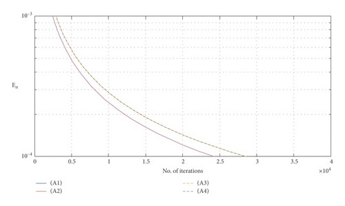
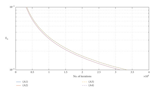
Example 2. In this example, we consider algorithm (23) for solving test problem (25), where N = 5 and M = 4. Let , , φ, a, and A be as in Example 1. In the numerical experiment, we take the stopping criterion En < 10−4. The numerical results are listed in Table 2 with different cases of P1 and P2. In Figures 3 and 4, we present the graphs illustrating the number of iterations for all cases of P1 and P2 using the stopping criterion as above with the different initial points appeared in Table 2. Moreover, Table 3 shows the effect of different choices of γ.
| Initial point | A1 | A2 | A3 | A4 | |
|---|---|---|---|---|---|
| (−2,1)T | n | 28577 | 24264 | 28577 | 24264 |
| s | 1.491225 | 1.355074 | 1.534414 | 1.282528 | |
| (1,3)T | n | 33407 | 31438 | 33407 | 31438 |
| s | 1.746868 | 1.693069 | 1.816897 | 1.690618 | |


| γ | 0.1 | 0.2 | 0.3 | |
|---|---|---|---|---|
| (−2,1)T | n | 9675 | 19200 | 28577 |
| s | 0.669508 | 1.245136 | 1.666702 | |
| (1,3)T | n | 11311 | 22447 | 33407 |
| s | 0.764536 | 1.372600 | 1.958486 | |
Remark 2. We observe from the numerical analysis of Table 2 that algorithm (23) has the fastest convergence when P1 and P2 satisfy (A4) and the slowest convergence when P1 and P2 satisfy (A3). Moreover, we require less iteration steps and CPU times for convergence when γ is chosen very small and close to zero.
Conflicts of Interest
The authors declare that there are no conflicts of interest.
Acknowledgments
The first author is thankful to the Science Achievement Scholarship of Thailand. The authors would like to thank the Department of Mathematics, Faculty of Science, Naresuan University (grant no. R2564E049), for the support.
Open Research
Data Availability
No data were used to support this study.


