Lowering Nitrogen Oxide Emissions in a Coal-Powered 1000-MW Boiler
Abstract
Burning of coal in power plants produces excessive nitrogen oxide (NOx) emissions, which endanger people’s health. Proven and effective methods are highly needed to reduce NOx emissions. This paper constructs an echo state network (ESN) model of the interaction between NOx emissions and the operational parameters in terms of real historical data. The grey wolf optimization (GWO) algorithm is employed to improve the ESN model accuracy. The operational parameters are subsequently optimized via the GWO algorithm to finally cut down the NOx emissions. The experimental results show that the ESN model of the NOx emissions is more accurate than both of the LSTM and ELM models. The simulation results show NOx emission reduction in three selected cases by 16.5%, 15.6%, and 10.2%, respectively.
1. Introduction
The energy statistics in China show that 59.2% of electrical energy comes from thermal electricity. This figure is just one percentage point lower than it was a year ago. The proportion of nonfossil energy sources (such as wind power, photoelectricity, and nuclear power) have increased recently, accounting now for nearly 41% of the total energy. In fact, the rapid development of new energy sources greatly affects the modes of operation of thermal power plants. Because of the uncertainty in energy supplies from wind and solar sources, thermal power plants must compensate for any failure in meeting grid demand. However, constant load changes pose a great challenge for energy conservation and emission reduction. According to new environmental standards in China, the emission of nitrogen oxide (NOx) pollutants from boilers fueled by burning coal must be below 50 milligrams (mg) per standard or normal cubic meters (Nm3) with a reference oxygen (O2) content of 6%. Therefore, a new operation mode for reducing NOx emissions should be proposed. Most of the coal-fueled power plants have already been equipped with selective catalyst reduction (SCR) modules. With the help of a catalyst, such modules turn NOx into diatomic nitrogen (N2) and water (H2O). However, too little catalytic material will not adequately reduce the emissions, while too much catalytic material will increase ammonia escape and even block the air preheater [1]. Alternatively, combustion optimization is typically used as a key process for guaranteeing lower NOx emissions with no additional modifications. Generally, an optimization method consists of two parts: constructing a prediction model and optimizing the operational parameters. However, the NOx emissions are interrelated with many operational parameters because of the complexity of the combustion process. Accurate modeling of NOx emissions can be hardly established with conventional methods. Fortunately, the emergence of machine learning techniques presents an alternative effective way for building NOx emission models. Several NOx modeling methods have been recently proposed. For instance, Zhou et al. [2] created a NOx emission model utilizing artificial neural networks (ANNs) and genetic algorithms (GA) for a pulverized coal-fired boiler of a large capacity. Ilamathi et al. [3] combined ANN and GA techniques and optimized the operational parameters for NOx emission prediction and reduction in a pulverized coal-fired boiler of a 210 MW capacity. Chu et al. [4] established an ANN model that enabled a reduction of NOx production. Unfortunately, an ideal ANN model should be trained with highly diverse examples, and ANN is vulnerable to overfitting and poor generalization. Three decades ago, support vector regression (SVR) methods started to compete with the ANN ones in modeling. In particular, the least-square support vector machines (LSSVM) emerged as a more effective variant of the standard support vector machines (SVM). In recent years, SVM and the LSSVM methods have been introduced as effective tools for modeling NOx emissions. Wu et al. [5] employed SVR for modeling the emissions of nitrogen oxides as well as carbon burnout of a coal-fired boiler of a 300 MW capacity. Tang et al. [6] employed the LSSVM for modeling the emissions of nitrogen oxides and utilized particle swarm optimization (PSO) to improve model accuracy. Lv et al. [7, 8] introduced a novel LSSVM model for NOx emission prediction and obtained results showing that this LSSVM model maintains good prediction accuracy. Li et al. [9] applied the SVM to establish a NOx emission prediction model, whose parameters were optimized by an enhanced PSO algorithm. Wang et al. [10] employed a LSSVM to model the emissions of nitrogen oxides for a 1000-MW once-through boiler. Fan et al. [11] fused a continuous restricted Boltzmann machine (CRBM) with SVR to model NOx emissions. Zhen et al. [12] addressed this modeling problem by integrating the LSSVM with a whale optimization algorithm (WOA). The WOA is used to optimize the kernel function width and penalty factor of the LSSVM. The simulation results showed that this method had stable, high-precision simulation performance. Apart from ANNs and SVMs, extreme learning machines (ELMs) have also been employed for modeling the emissions of nitrogen oxides. Li et al. [13] introduced ELMs as a tool for building a model for the emissions of nitrogen oxides, and they proposed an enhanced algorithm of teaching-learning-based optimization (I-TLBO), in order to fine-tune the ELM parameters and improve the modeling accuracy. Dong et al. [14] proposed the combination of partial least squares (PLS) and ELMs to assess NOx emissions of a 1000-MW once-through boiler. Recently, deep learning has been applied in image diagnosis [15], human activity recognition [16], and 5G networks [17]. The emergence of deep learning has led to the use of the long short-term memory (LSTM) architectures in modeling NOx emissions. Yang et al. [18] adopted the LSTM neural network to predict NOx emissions. Compared with the recurrent neural network (RNN) model, the LSTM model generally demonstrated a higher accuracy. Tan et al. [1] applied the LSTM approach for dynamic modeling of the NOx emissions of a 660-MW coal-fired boiler. They asserted that the LSTM model outperforms the SVM approach. Xie et al. [19] introduced a novel LSTM method with a new attention mechanism to model the NOx emissions, and the results demonstrated a superior prediction accuracy of the NOx emissions.
Additionally, any desirable combustion optimization algorithm should exhibit rapid convergence and high-quality solutions. Indeed, the past two decades witnessed a dramatic increase in the popularity of metaheuristic optimization techniques, and especially the application of these techniques in combustion optimization. For example, Zhou et al. [20] employed a PSO algorithm to optimize the parameters of a SVR model of NOx emissions. The emissions could be reduced by 32.67% and 16.3%, respectively, when the model was exploited with and without optimization. Wei et al. [21] utilized quantum genetic algorithms (QGA) together with simulated-annealing genetic algorithms (SAGA) for the optimization of the operating parameters, and hence the reduction of the emissions of nitrogen oxides. An improved flower pollination algorithm (IFPA) [22] was used to optimize hyper-parameters. An artificial bee colony (ABC) algorithm [23, 24] was also used for modeling and optimization of coal-fired boilers.
Notwithstanding the dramatic success achieved so far by methods for combustion optimization in lowering the emissions of nitrogen oxides, more improvements are still needed. A candidate for achieving such improvements is a novel variant of recurrent networks, namely, the echo state networks (ESNs). These networks enjoy the advantages of simplicity and high accuracy, which enable them to find diverse applications such as the prediction of the remaining useful life (RUL) [25], energy prediction [26], and anomaly detection [27]. Nevertheless, ESNs have been hardly applied for modeling the emissions of nitrogen oxides. Moreover, the grey wolf optimization (GWO) method has been introduced and subsequently employed in tackling real-world optimization problems [28–30]. In this work, the GWO method is used to optimize both the ESN model parameters and the operational parameters with the target of lowering the emissions of nitrogen oxides.
In summary, we introduce a combustion optimization method to lower the emissions of nitrogen oxides for a coal boiler that has a 1000-MW capacity. We introduced the ESN for modeling the NOx emissions and compared the ESN model against the ELM and LSTM ones. Meanwhile, we used the GWO algorithm for optimizing the operational parameters and lowering the emissions of nitrogen oxides based on an earlier NOx emission model. For validating the proposed method, we selected three typical values of the boiler maximum continuous rating (BMCR), namely, 100%, 90%, and 80%, for optimization by the GWO algorithm.
2. Methodology
2.1. Echo State Networks
An echo state network (ESN) is a variant of recurrent neural networks (RNN), basically distinguished via its dynamic reservoir (DR) within its sparsely connected hidden layer. The purpose of this reservoir is to allow the input sequence to expand nonlinearly. The ESN essentially has an RNN architecture, where the input and output layers are detached from each other by recurrent connected units. The network is trained through an initial random choice of both the input and the reservoir weights, followed by fixing these weights through the overall training process. Any feedback signals from the outputs to the reservoir are initially set randomly and then kept fixed in a similar fashion. The supervised training of the network updates only the readout weights. The basic architecture of an ESN is depicted in Figure 1.
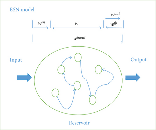
The two functions, f and fout, are activation functions that can be either of the hyperbolic tangent (tanh) or linear types. As we have formerly asserted, the backward weights and those of the input and the reservoir are initially set randomly and then kept fixed. In order to define these weight matrices, we should consider certain metrics. In particular, we should carefully define the input scaling and the connectivity rate from the outset. Here, the term “input scaling” refers to the weight value range, while the term “connectivity” indicates how many connections we need to define for each matrix. We can guarantee that the network will not be driven by the internal or reservoir dynamics, provided the aforementioned factors are well set.
2.2. Grey Wolf Optimizer
The value of a is iteratively decreased in a linear fashion from 2 to 0, and r1 and r2 are numbers randomly generated from the unit interval [0,1]. Equations (3) and (4) describe how grey wolves update their positions, while still encircling their preys.
2.3. A Hybrid Optimization Technique Integrating ESN and GWO
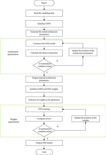
For applying the ESN model, we must properly specify network parameters and designations such as the infrastructure of the reservoir, and also the network weights and connections. However, even if we apply the settings recommended by Jaeger [32] for the reservoir initialization stage, we cannot guarantee that the ESN model will suit the intended application. We should realize that the ESN performance is essentially associated with the reservoir design, and if we conceive this well, then we can aspire to obtain satisfactory results. We might repeat the tests hoping to acquire good design scenarios. However, we can never be certain about achieving optimal scenarios. Anyhow, the design procedure should involve a few parameters, including the number of neurons within the network (NN), the connectivity rate of the network (RR), the feedback rate (FR), and the input connectivity rate (IR). Meanwhile, since not all the weights are being updated as part of the training process, pretraining is needed to suit the targeted task. The GWO algorithm should be used in such a way that it serves as an optimization algorithm. Figure 2 shows a flowchart of the proposed model for nitrogen oxide emissions. The following steps describe the specific modeling procedure:
Step 1. Enter the input data.
Step 2. Initialize the a, A, and C parameters of the GWO algorithm.
Step 3. Set the initial architecture parameters including NN, RR, FR, and IR.
Step 4. Use the architecture parameters to establish the ESN model.
Step 5. Calculate the emissions of nitrogen oxides for different architecture parameters and use the mean absolute error as the corresponding fitness measure.
Step 6. Obtain the minimum fitness values for all architecture parameters.
Step 7. If the obtained minimum fitness values satisfy the requirements of model accuracy, then jump to Step 9. Otherwise, continue.
Step 8. Use Equation (9) to update the positions, increment the counter for the number of iterations, and then return to Step 4.
Step 9. Output the parameters of the optimal architecture.
Step 10. Initialize a, A, and C parameters in the GWO and ESN weights.
Step 11. Select the weights to be optimized.
Step 12. Train the ESN model.
Step 13. Compute the error.
Step 14. If the error satisfies the model accuracy requirement, then jump to Step 16. Else, continue.
Step 15. Use Equation (9) to update the positions, increment the counter for the number of iterations, and then return to Step 12.
Step 16. Output the ESN model.
2.4. Optimizing the Operational Parameters Using GWO
We seek to establish a model for nitrogen oxide emissions, through which we can assess how the operational parameters are relevant to these emissions. As a bonus, emission reduction can be achieved by fine-tuning the operational parameters of the aforementioned model. We selected two of the most sensitive sets of operational parameters herein as candidates for potential change. These are parameters of the separated overfire air (SOFA) flow rate (four parameters) and the secondary air-damper opening percentage (six parameters). We carefully identified ranges for possibly adjusting these changeable parameters. We based our range selections on the standard operation habits and the accumulated experience of the operators and engineers. The following steps describe our procedure in detail:
Step 1. Enter the input data.
Step 2. Obtain the initial values for the a, A, and C parameters in the GWO algorithm.
Step 3. Generate the initial operational parameters.
Step 4. Calculate the nitrogen oxide emissions for the different operational parameters and the corresponding errors.
Step 5. If the minimum error values satisfy the production requirements, then jump to Step 7, or else continue.
Step 6. Use Equation (9) to update the positions, increment the counter for the number of iterations, and then return to Step 4.
Step 7. Produce the optimal operational parameters as the final output.
3. Experimental Setup, Results, and Discussion
We obtained more than 5,000 patterns from the distributed control system (DCS) of the coal-fueled boiler (the power plant) and employed a sampling interval of 1 minute. Table 1 lists the properties of the coal fueling the power plant.
| Explanation | Unit | Value |
|---|---|---|
| Carbon | % | 61.7 |
| Oxygen | % | 8.56 |
| Hydrogen | % | 3.67 |
| Nitrogen | % | 1.12 |
| Sulfur | % | 0.60 |
| Ash | % | 8.80 |
| Moisture | % | 15.55 |
| Volatile component | % | 26.50 |
| Quantity of produced heat | KJ/kg | 23442 |
The model employed twenty variables that can be detailed as follows: unit load, total coal flow rate, total airflow rate, feed-water flow, main steam pressure, main steam temperature, water coal ratio, boiler tail flue temperature, separated overfire air (SOFA) flow rate (four variables), secondary air damper opening percentage (six variables), flue gas oxygen content, and NOx emissions. The input variables were selected according to basic boiler knowledge and the engineers’ suggestions. In this work, all data of nitrogen oxide emissions is presented on the basis of a dry gas at 6% O2. Data preprocessing was conducted prior to the modeling process. First, noise and outlier removal operations were conducted to enhance the quality of the coarse or raw sampling data. Then, we removed all operational variables that do not experience any change during sampling. We also calculated the average values for variables with multiple measurements.
3.1. Performance Indices
3.2. Modeling of NOx Emissions
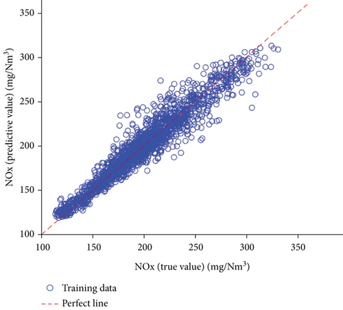
Figure 3 illustrates both the predicted and measured training data samples for the emissions of the nitrogen oxides according to the established ESN model. The dotted red straight line is the perfect line which indicates the equivalence of the predicted and measured values. The blue points indicate the ESN prediction results, associated with the measurements. All data points are almost distributed or scattered along the perfect line. Based on our calculations, the MAPE for the training dataset was only 4%, while the coefficient of determination (R2) was 0.91. This shows that the ESN is highly suitable for modeling the nitrogen oxide emissions.
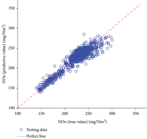
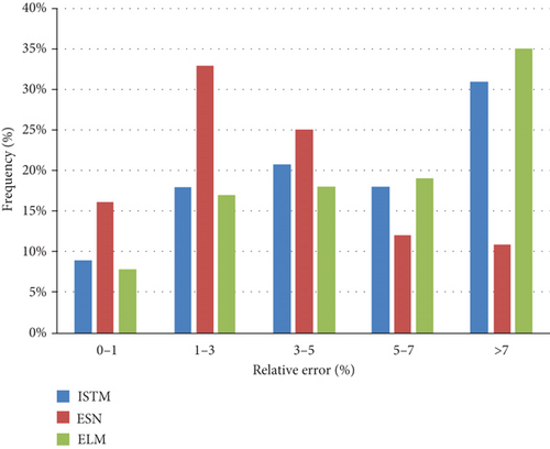
After we trained the NOx model on a part of the dataset, we employed the remaining part of the dataset to assess the performance of the model. Figure 4 presents the prediction results of 1000 test cases. Like the situation in Figure 3, the points in Figure 4 are also nearly aligned with the perfect line. This means that the prediction results are in good agreement with the measurements. Figure 5 shows the ESN-based distribution of the relative test errors. Among 1000 test samples, 74% of the relative errors were below 5%. The RMSE and R2 were also calculated and were found to be 10.527 and 0.86, respectively. These results enable us to conclude that the proposed ESN model is accurate in its NOx emission prediction.
3.3. Performance Comparison with LSTM and ELM
To further demonstrate the superiority of the performance of the ESN model, we compared the ESN model outcomes with those of the widely used ELM model and the LSTM model.
The ELM model is an effective machine learning method, which generally demonstrates superior accuracy and generalization performance in comparison with the conventional SVM and LS-SVM methods. To realize the actual modeling process, we employed a Matlab implementation of the ELM algorithm with a sigmoidal transfer function. A trial-and-error scheme was followed to set the number of neurons. The LSTM architecture is a RNN variant, which includes a single input layer, a single hidden layer, and also a single output layer, such that the dropout is set after the hidden LSTM layer.
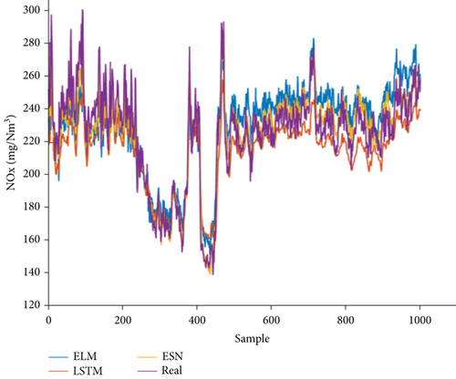
Figures 5 and 6 and Table 2 provide a brief outline of the performance of each of the aforementioned three different models. Figure 6 asserts that each of the three prediction curves follows the real-data direction and that each of the three algorithms can be employed to successfully predict the emissions of nitrogen oxides. However, the results in Table 2 suggest that the prediction accuracy of either LSTM or ESN exceeds that of ELM. This indicates that the RNN prediction accuracy strongly exceeds that of a conventional model. Figure 5 illustrates the relative test error distributions, showing that the majority of the ESN errors are within 5%. Table 2 lists the MAPE, MAE, RMSE, and R2 indicators for the test dataset with different models. The ELM model, which represents a conventional machine learning approach, is clearly underperformed by the ESN and LSTM models. Indeed, the ELM produces the most inaccurate results on three of the four criteria. The MAPE, MAE, and R2 of the LSTM are better than those of the ELM, but the RMSE of the LSTM is slightly inferior to the RMSE of the ELM. The MAPE, MAE, RMSE, and R2 criteria of the ESN model are better than the performance indices of the other two models. This indicates that the ESN model is a promising alternative for achieving the required accuracy when dealing with models of nitrogen oxide emissions.
| Model | MAPE | MAE | RMSE | R2 |
|---|---|---|---|---|
| ESN | 0.0353 | 8.052 | 10.527 | 0.868 |
| LSTM | 0.0559 | 12.89 | 16.042 | 0.867 |
| ELM | 0.0589 | 13.23 | 15.853 | 0.735 |
3.4. Combustion Optimization with the GWO Algorithm
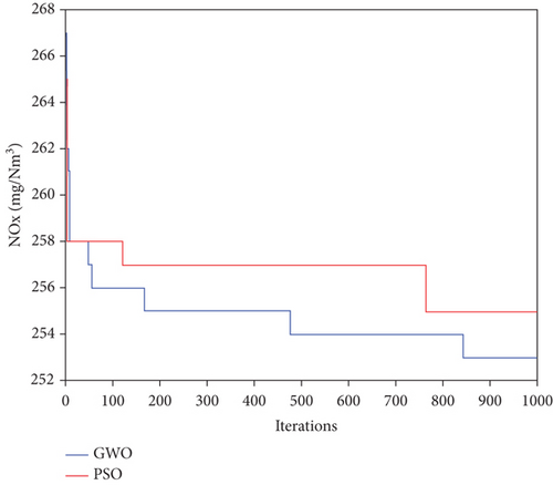
In this paper, we selected three standard optimization cases according to the boiler maximum continuous rating (BMCR). The values for this rating were 100% BMCR (Case 1), 90% BMCR (Case 2), and 80% BMCR (Case 3). The original nitrogen oxide emissions for these three selected cases were, respectively, 303, 270, and 216 mg/Nm3. We also selected two sets of parameters (namely, the secondary air damper opening percentage (x1, x2, x3, x4, x5, x6) and the SOFA flow rate (x7, x8, x9, x10) as design variables to be optimized by the GWO algorithm. We determined these variables and their ranges to be conforming to the regular operation habits and the accumulated experience of operators and engineers. Figure 7 illustrates the search process employed in Case 1. This search process is a convergent one with an extremely fast speed of convergence. The simulation results indicate that the predicted emissions of nitrogen oxides were lowered to approximately 253, 228, and 194 mg/Nm3 from their original values of 303, 270, and 216 mg/Nm3, respectively. Therefore, the ratios of reduction amounted to percentages of 16.5%, 15.6%, and 10.2%, respectively. Table 3 lists both the original and optimized parameters. In order to verify the GWO performance, we compared the widely used PSO algorithm and the present GWO algorithm. To achieve this comparison, we repeated both algorithms thirty times with an eye to optimize Case 1. Figure 7 indicates that both the PSO and GWO algorithms can dramatically lower the emissions of the nitrogen oxide pollutants. On average, the GWO optimization results are superior to those of the PSO one. This means that the GWO algorithm can offer solutions of a higher quality and better stability. In short, the GWO algorithm may offer a better alternative for combustion optimization.
| x1 (%) | x2 (%) | x3 (%) | x4 (%) | x5 (%) | x6 (%) | x7 (t/h) | x8 (t/h) | x9 (t/h) | x10 (t/h) | NOx (mg/Nm3) | ||
|---|---|---|---|---|---|---|---|---|---|---|---|---|
| Case 1 | Original | 14 | 59 | 37 | 60 | 41 | 70 | 101 | 95 | 129 | 77 | 303 |
| Optimized | 15 | 53 | 38 | 66 | 42 | 75 | 127 | 110 | 147 | 90 | 253 | |
| Case 2 | Original | 14 | 65 | 31 | 65 | 32 | 72 | 141 | 101 | 141 | 82 | 270 |
| Optimized | 14 | 54 | 28 | 79 | 39 | 86 | 204 | 137 | 186 | 116 | 228 | |
| Case 3 | Original | 14 | 79 | 49 | 79 | 49 | 79 | 153 | 128 | 173 | 105 | 216 |
| Optimized | 15 | 73 | 50 | 84 | 54 | 81 | 179 | 139 | 181 | 114 | 194 |
4. Conclusions
We consider two important steps towards optimizing combustion processes to achieve low emissions of nitrogen oxides. These steps are modeling of NOx emissions and optimization of the pertinent operational parameters. In this work, we introduce a novel approach, which combines the ESN and GWO algorithms to model the emissions of nitrogen oxides and optimize the pertinent operational parameters in a coal-fueled boiler of a 1000 MW capacity. We utilized the ESN algorithm to model the NOx emissions of this boiler and, further, utilized this model to optimize the relevant operational parameters through the application of the GWO algorithm. We finally managed to lower the nitrogen oxide emissions through the adjustment of the pertinent parameters to their optimal values. We found the values predicted by the ESN model for the NOx emissions to be consistent with their measured values. We obtained a mean absolute error (MAE) of the test data that was as low as 3.5%. In comparison with the LSTM and the ELM algorithms, the ESN algorithm is more successful in the modeling of nitrogen oxide emissions due to its strong generalization capability. We selected a secondary opening percentage and a separated overfire air (SOFA) flow rate from three typical cases for optimization by the GWO algorithm. Our simulation results for the three selected cases indicated that the nitrogen oxide emissions were lowered by 16.5%, 15.6%, and 10.2%, respectively. Compared with the widely used PSO, our approach lowers the nitrogen oxide emissions within any specified time and increases the solution stability. In summary, our proposed combination of the ESN and GWO algorithms can model and lower the emissions of nitrogen oxides for coal-fired boilers. Our approach is more powerful and effective than other modeling approaches such as the LSTM and ELM algorithms and other optimization approaches such as the PSO algorithm.
Conflicts of Interest
The authors declare no conflict of interest.
Authors’ Contributions
X. J. Chen designed the research and the article structure and revised the manuscript. H. Y. Zhang carried out the experiments and revised the manuscript. H. W. Qin revised the manuscript. All authors read and approved the final paper.
Open Research
Data Availability
The data employed in creating our model pertain to a 1000 MW ultra-supercritical once-through boiler with variable pressure and octagonal-inverse double tangential firing.


