Mixed estimators in nonparametric regression have been developed in models with one response. The biresponse cases with different patterns among predictor variables that tend to be mixed estimators are often encountered. Therefore, in this article, we propose a biresponse nonparametric regression model with mixed spline smoothing and kernel estimators. This mixed estimator is suitable for modeling biresponse data with several patterns (response vs. predictors) that tend to change at certain subintervals such as the spline smoothing pattern, and other patterns that tend to be random are commonly modeled using kernel regression. The mixed estimator is obtained through two-stage estimation, i.e., penalized weighted least square (PWLS) and weighted least square (WLS). Furthermore, the proposed biresponse modeling with mixed estimators is validated using simulation data. This estimator is also applied to the percentage of the poor population and human development index data. The results show that the proposed model can be appropriately implemented and gives satisfactory results.

1. Introduction

One of the most popular statistical methods often used for prediction is regression analysis. Regression analysis is commonly used to determine the functional relationship between independent variables (predictors) and dependent variables (responses) [1]. Functional relationships between predictor variables and response variables can have clear or unknown patterns; if these relationships have unknown patterns, the appropriate type of regression analysis is nonparametric regression [2]. In the nonparametric regression, the regression curve is assumed to be smooth. This regression has high flexibility because the data can drive to estimate its own regression curve without subjectivity from the researcher [3]. Researchers have proposed methods for estimating nonparametric regression functions such as spline, kernel, and Fourier series functions. The spline nonparametric regression has been developed by Eubank [3], Becher et al. [4], and Wang et al. [5]. Hall and Huang [6], Okumura and Naito [7], Du et al. [8], Chamidah and Saifudin [9], and Erçelik and Nadar [10] developed kernel nonparametric regression. Bilodeau [11] and Amato et al. [12] estimated the nonparametric regression function with the Fourier series function.

In applying nonparametric regression modeling, researchers sometimes assume that each predictor variable has the same pattern. Although there are often real cases with different patterns between the response and each predictor, if the researcher still insists on applying one type of estimator to all predictor variables, the estimation results can be inaccurate and produce a large error. Researchers have begun to develop nonparametric regression with a mixed estimator, including Hidayat et al. [13], Mariati et al. [14], and Octavanny et al. [15]. These mixed estimators are formed by referring to the idea of semiparametric regression. The semiparametric regression model is an additive regression model that consists of a parametric component and a nonparametric component; see the work of Green and Yandell [16], Roozbeh and Arashi [17], and Roozbeh and Najarian [18]. In these mixed estimators, the additive model concept in semiparametric regression is adapted by modification using two different nonparametric components. However, these mixed estimators only use one response variable, even though some biresponse cases also have different patterns among the predictor variables. At present, nonparametric regression studies with mixed estimators for biresponse cases have never been developed. Therefore, this study develops a new theory about the mixed estimator of spline smoothing and kernel in biresponse nonparametric regression. This mixed estimator is the development of the mixed estimator proposed by Hidayat et al. [13] that the kernel estimator is considered to be fixed, while the kernel function in this paper is estimated. In addition, this new mixed estimator can be applied for biresponse cases. This mixed estimator is obtained through a two-stage estimation. The first stage of estimation uses the penalized weighted least square (PWLS) to obtain the spline smoothing component, followed by the second stage that employs the weighted least-square (WLS) estimation method to estimate the kernel component.

The spline smoothing estimator is very dependent on the smoothing parameter, while the kernel estimator is very dependent on the bandwidth parameter. These smoothing and bandwidth parameters are tuning parameters. The optimal value of these parameters will produce the best regression model. In nonparametric and semiparametric regression, there are several methods to determine the optimal parameter value to obtain the best regression model. Some of the popular methods are the cross-validation (CV) and generalized cross-validation (GCV) methods. The CV method is a method of selecting the best model based on the best predictive ability from all the different datasets. This method is widely used, but the calculation of this method will become more complex as the number of datasets increases. In addition, for partial linear models including mixed estimator models, the one-out crossover method tends to be time consuming even for moderate sample sizes [19]. Craven and Wahba [20] modified the CV method to make the calculation simpler, and the result of this modification is called the GCV method. This method is widely used by researchers because it has several advantages. The advantages of the GCV method include the following: simple and efficient in calculation, invariant to transformation, and does not require variant information. This method also has the advantage of optimal asymptotic properties over other methods [21, 22]. Some researchers develop specific GCV methods according to the model in their research such as the GCV for semiparametric ridge regression with kernel smoothing [23–25]; also, several types of GCV were developed for uniresponse nonparametric regression with mixed estimators including the mixed estimator of spline smoothing and kernel [13], mixed estimator of spline smoothing and Fourier series [14], and mixed estimator of truncated spline and fourier series for longitudinal data [15]. Therefore, in this study, the determination of the best model was carried out using the GCV method which was developed specifically for the mixed estimator of spline smoothing and kernel in biresponse nonparametric regression.

Next, the proposed mixed estimator is applied to the simulation data. The formula for generating data contains two different functions to represent two different patterns of predictor variables. This estimator is also implemented to model to the percentage of the poor population and human development index data in Papua Province, Indonesia. Empirical results indicate that the proposed mixed estimator performs very well for modeling the data with two different patterns. One pattern (response vs. predictors) tends to change at certain subintervals, and another pattern appears to be random, which are commonly modeled using kernel regression.

The rest of this paper is organized as follows: In Section 2, we present the materials and methods about the two-stage estimation method, i.e., the PWLS and followed by the WLS. The proposed mixed spline smoothing and kernel estimator in biresponse nonparametric regression is explained in Section 3.1. The selection of smoothing and bandwidth parameters using generalized cross validation (GCV) is described in Section 3.2. The simulation study and real data analysis are conducted to illustrate the performance of the proposed biresponse mixed estimator in Sections 3.3 and 3.4. The conclusions and further research are presented in the last section.

2. Materials and Methods

The paired data (y_1i, y_2i, x_i, t_i) are given, where some predictor variables have a pattern that changes at certain subintervals, and the remaining predictors have a typically random pattern. This work adopts the idea of the semiparametric regression model developed by Green and Yandell [16], which employed an additive model to combine parametric and nonparametric models. Thus, the additive model for nonparametric biresponse regression with two different estimators can be formulated as follows:

(1)

where μ_hi(x_i, t_i) is a regression curve. In the biresponse cases, if y_hi and

are in pairs, then there is a correlation between the error of h-response and error of h’-response (h ≠ h^′). Error correlation between responses can be defined as

, where

i = 1,2, …, n; h = 1,2; h ≠ h^′ [5].

Each regression curve μ_hi(x_i, t_i) is assumed to be unknown and additive so that it can be written as

(2)

If equation (2) is substituted into equation (1), then equation (1) can be expressed in the following vector form:

(3)

The component of the regression curve g is approximated by the spline smoothing function, which is assumed to be smooth and contained in the Sobolev space

, while the component of the regression curve f is approximated by the kernel function. Mixed spline smoothing and kernel estimator in biresponse nonparametric regression can be obtained through the two-stage estimation method. The first stage is performed by estimating the spline smoothing component using the PWLS method, and the second stage is estimating the kernel component using the WLS method. To estimate the spline smoothing part, equation (3) is modified to the following form:

(4)

where z = y − f.

Estimation of the spline smoothing component

can be performed by applying PWLS optimization to equation (5), and then, the estimation results in the first stage are substituted into equation (3).

(5)

The estimation of the kernel component

is obtained in the second stage estimation using WLS optimization in equation (6). Furthermore, the results of the two-stage estimations are substituted into equation (3) to obtain the mixed spline smoothing and kernel estimator in biresponse nonparametric regression.

(6)

where K_α(t₀) is a weighting matrix for the kernel estimator and M⁻¹ in equations (5) and (6) is a weighting matrix for the biresponse nonparametric regression like in the work of Wang et al. [5].

3. Results and Discussion

3.1. Mixed Spline Smoothing and Kernel Estimator in Biresponse Nonparametric Regression

Before conducting the estimation to obtain biresponse mixed spline smoothing and kernel estimator, it is necessary to obtain the function form for each component of this mixed estimator. The structure of the spline smoothing component is explained in Lemma 1, while the kernel component is explained in Lemma 2.

Lemma 1. If the regression curve g is assumed to be smooth and contained in the Sobolev space [22], then the function form of the spline smoothing component in the biresponse nonparametric regression can be stated as

(7)

with

(8)

where

(9)

{τ_h1, τ_h2, …, τ_hm} and {β_h1, β_h2, …, β_hn} are bases of spaces in the Sobolev space.

Proof. If g_h; h = 1,2 is a function lying in Hilbert space H, the H space can be decomposed into a direct sum of two spaces H₀ and H₁ where H = H₀ ⊕ H₁ and H₀ ⊥ H₁. If {τ_h1, τ_h2, …, τ_hm} is the basis in H₀ and {β_h1, β_h2, …, β_hn} is the basis in H₁, according to Wahba [22], for each function g_h ∈ H with u_h ∈ H₀ and v_h ∈ H₁, we obtain

(10)

where

(11)

Equation (10) is a limited linear function in H space and g_h ∈ H; therefore, equation (10) can be stated as

(12)

and using inner product properties, equation (12) can be written as

(13)

and for each response with all observations (i = 1,2,3, …, n), we can obtain the following vector g_h:

(14)

where

(15)

where

and 〈η_hi, β_hi〉 are equal to

with

i = 1,2, …, n; i^′ = 1,2, …, n; s = 1,2, …, m; h = 1,2

Therefore, for all responses (h = 1,2), we can obtain the function form of the spline smoothing component in the biresponse regression curve as follows:

(16)

Lemma 2. If the regression curve f is approached by the kernel function, then the function form of kernel component in the biresponse nonparametric regression can be expressed as

(17)

where

(18)

with

(19)

The function f_h(t_i); h = 1,2; i = 1,2, …, n is approached by the Taylor series with t around t₀.

Proof. The form of the regression function f is derived from the component f_h(t_i) in equation (2). The form of the function is unknown and approached using the kernel estimator. The function f_h(t_i) for h = 1,2 can be approached by the Taylor series with t around t₀ as follows [9]:

(20)

and if

, then equation (20) can be stated as

(21)

where t ∈ (t₀ − α, t₀ + α), t₀ is the predictor value for prediction.

The kernel estimator can be obtained when the polynomial order m_h = 0; h = 1,2. Therefore, the function form for each response involving all observations can be stated as

(22)

Then, we can obtain the function form of component f in biresponse nonparametric regression as follows:

(23)

where

;

Theorem 1. The biresponse nonparametric regression model is given in equation (1), where each component of the regression curve is additive as stated in equation (2). The function form of the g component is presented in Lemma 1, and the function form of the f component is presented in Lemma 2. Using PWLS in the first-stage estimation and WLS in the second-stage estimation, the mixed spline smoothing and kernel estimator in biresponse nonparametric regression is obtained as follows:

(24)

where

(25)

while

is obtained from the first-stage estimation and

is obtained from the second-stage estimation.

Proof. The first-stage estimation on the mixed spline smoothing and kernel estimator in biresponse nonparametric regression is performed by estimating the spline smoothing component using the PWLS in equation (5). The penalty component in equation (5) can be obtained through the following decomposition [26]:

(26)

where P₁ is the orthogonal projection of g_h to H₁ in H space. By substituting equation (26) into the penalty component, we obtain

(27)

and furthermore, the PWLS optimization in equation (5) can be written in matrix notation as follows:

(28)

The solution for the PWLS optimization can be obtained from the partial derivative Q(c, d) by c and d. The partial derivative Q(c, d) by c results as follows:

(29)

if R = M⁻¹V + 2nΛ; thus, we can obtain

(30)

The partial derivative of Q(c, d) by d gives the result

(31)

and by substituting equation (30) into equation (31), we can obtain

(32)

considering that R = M⁻¹V + 2nΛ so matrix V can be stated as V=M(R − 2nΛ); then, we can modify

(33)

Equation (33) is substituted into equation (32), and then, we solve it and get the following result:

(34)

Furthermore, by substituting equation (34) to equation (30), we obtain

(35)

and are substituted into the function form of the spline smoothing component in equation (16), and then, the following spline smoothing estimator component in the biresponse nonparametric regression model is obtained:

(36)

where

(37)

Because z = y − f, the first-stage estimation results can be stated as

(38)

and remember that z = g + ε; then, the model in equation (4) can be written as

(39)

In the second stage of estimation, the function f as the kernel component on a mixed spline smoothing and kernel estimator in biresponse nonparametric regression is estimated using the WLS method with the following formula:

(40)

where M⁻¹ is a weighting matrix for biresponse nonparametric regression and K_α(t₀) is a weighting for the kernel estimator with the following structure:

(41)

where

and

is the kernel function.

By substituting the results of the first-stage estimation (38) and the function form f (Lemma 2) into the model of the mixed estimator (equation (3)), the error of this mixed estimator model can be written as follows:

(42)

Furthermore, by supposing D = M⁻¹K_α(t₀) and substituting equation (42) into equation (40), we can get the following equation for WLS optimization:

(43)

The solution for the WLS optimization can be obtained from the partial derivative Q(t₀) by ω₀(t₀). The optimization result is obtained as follows:

(44)

Therefore, the estimation for kernel estimator component can be written as

(45)

where

(46)

Based on the first-stage estimation results in equation (38) and the second-stage estimation results in equation (45), the estimation of the additive regression curve in equation (2) with the mixed spline smoothing and kernel estimator in biresponse nonparametric regression can be stated as

(47)

and we can write equation (47) as

(48)

where H(λ, α) = A(λ, α) − A(λ, α)B(λ, α) + B(λ, α).

3.2. Selection of Smoothing and Bandwidth Parameters

The best model for the biresponse mixed spline smoothing and kernel estimator depends on the optimal smoothing parameters (λ_opt) and optimal bandwidth parameters (α_opt), where λ and α are tuning parameters. These optimal parameters can be obtained from the model with the smallest generalized cross-validation (GCV) value, see [13–15, 23–25]. The GCV criteria are one of the methods to determine the best model in nonparametric regression [20]. The GCV formula for the mixed spline smoothing and kernel estimator in biresponse nonparametric regression (48) can be stated as follows:

(49)

3.3. Simulation Study

In this simulation, the mixed spline smoothing and kernel estimator in biresponse nonparametric regression, as formulated in equation (48), is applied to the simulation data. The simulation data are generated from a formula that contains two different functions, i.e., a polynomial function and an exponential function, to present two different patterns for each predictor. The polynomial function is used to generate spline smoothing-like patterns, and the exponential function is used to generate patterns in the data such as kernel. Using two response variables and two predictor variables, the formula for generating data is defined as follows:

(50)

with

(51)

The predictors are generated from x_i ~ U(0,2) and t_i ~ U(0,2) with the sample size n = 100, and the random errors ε_hi are generated from bivariate normal distributions with , and ρ = 0.6. The scatterplots of the simulated data are shown in Figure 1. It can be seen that the pattern between y₁, y₂ against x tends to change at certain subintervals such as the spline smoothing pattern, while the scatterplot between y₁, y₂ against t tends to have a random pattern that is commonly modeled with kernel regression.

Details are in the caption following the image — **Figure 1**
Open in figure viewer PowerPoint

Plots of the simulation data.

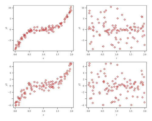
In this simulation, the Gaussian kernel was employed. Based on the empirical results from the two-stage estimation, we obtain combination values of the smoothing parameters (λ₁, λ₂) and bandwidth parameters (α₁, α₂) around the optimal values (Table 1). The exhibited results are a few of all combinations due to the limited space. The best model is chosen based on the smallest GCV value resulted from optimal smoothing parameters λ_1(opt) = 0.0002413 and λ_2(opt) = 0.0000899 along with optimal bandwidth parameters α_1(opt) = 2.396 and α_2(opt) = 2.416. This model produces the lowest GCV = 3.239 with R² = 99.91% and RMSE = 0.1045.

Table 1. Combination of smoothing (λ_h) and bandwidth (α_h) parameters with the GCV value.

λ₁	λ₂	α₁	α₂	GCV
0.002413	0.000899	23.96	24.16	13.123
0.0002413	0.0000899	23.96	24.16	3.397
0.002413	0.000899	2.396	2.416	12.143
0.0002413	0.0000899	2.396	2.416	3.239
0.00002413	0.00000899	2.396	2.416	5.739
0.0002413	0.0000899	0.2396	0.2416	11494.49
0.00002413	0.00000899	0.2396	0.2416	3130.825

The result of modeling simulation data using the mixed spline smoothing and kernel estimator is compared with modeling using either a spline smoothing estimator or kernel estimator only. The results of these models are presented in Table 2. From Table 2, we can find out the best model that gives the smallest GCV value is the model with the mixed spline smoothing and kernel estimator. Besides, this model has the largest R² and the lowest MSE value.

Table 2. Comparison between three estimators.

Model	Minimum GCV
Mixed spline smoothing and kernel	3.2392
Spline smoothing	4.6587
Kernel	4.4085

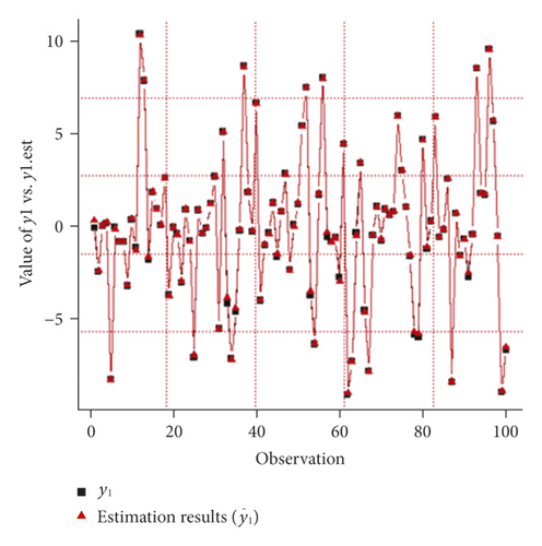
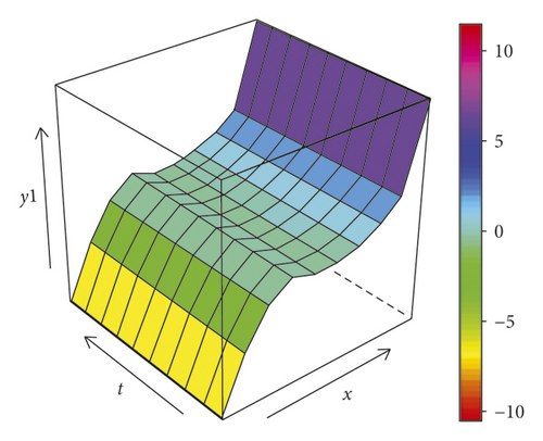
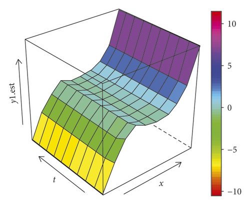
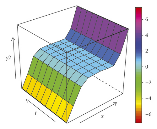
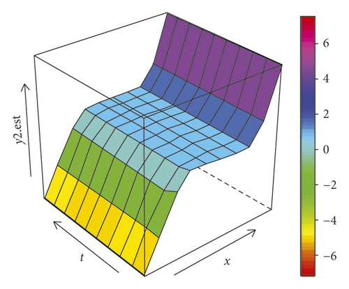
The plot between the estimation results and the original simulation data is presented in Figure 2, where the estimated values (red triangles) are very close to the original data (black squares). Thus, the proposed model and estimation procedure can be used to make a prediction correctly. Furthermore, on the left side of Figure 3, the surface plots are formed using equation (50), which is the equation for generating simulation data, whereas on the right side of Figure 3, there are two surface plots for each response which are formed from equation (48) where its parameters are estimated using two-stage estimation, i.e., the PWLS and WLS. The two sides of Figure 3 show that the plots appear to have similar surface shape. This evidence indicates that the estimation procedure proposed in equation (48) can be used appropriately to estimate the function generated from the simulation.

3.4. Data Application

The biresponse mixed spline smoothing and kernel estimator proposed in this paper is applied to regress the percentage of the poor population (PPP), as the first response, and human development index (HDI), as the second response, on several predictors. These two response variables are important because they are indicators of the success level of a country’s development. The adoption of biresponse modeling for the two variables considers the initial study that there is a negative correlation between PPP and HDI. If the PPP in a region is getting lower, the HDI in that region will be higher [27, 28].

Several variables that typically affect the two response variables are the gross regional domestic product (GRDP) and the population growth rate. Some researchers have pointed out several factors that can affect the PPP and HDI, including Grubaugh [29], who stated the variables that influence the growth of HDI in developing countries are population, population growth, and the initial level of the gross domestic product (GDP). Meanwhile, Mallick and Ghani [30] found that high population growth is the cause of poverty in Pakistan. While in North Sumatra Province, Indonesia, the GRDP and education level to university have a positive and significant influence in reducing the PPP [31]. Based on Malthus’s theory, poverty is considered as the impact of high population growth rates [32]. Also, additional life support needs are considered slower than population growth. A high increase in population growth will have an impact on decreasing the quality of natural resources and reducing the opportunity for people to access life-support facilities. This situation can reduce the quality of human life, and people will be challenged to live in prosperity. Rapid economic growth is one way to alleviate poverty [33]. The GDP or GRDP has a close relationship with economic growth because the economic growth of a region is related to an increase in production or an increase in income per capita. Besides, if the GRDP is higher, the income per capita in the region will increase and have an impact on increasing the ability of the community to meet their needs and improve their quality of life.

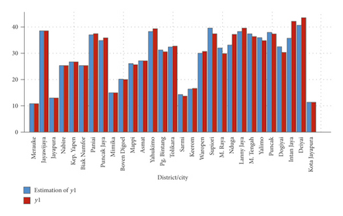
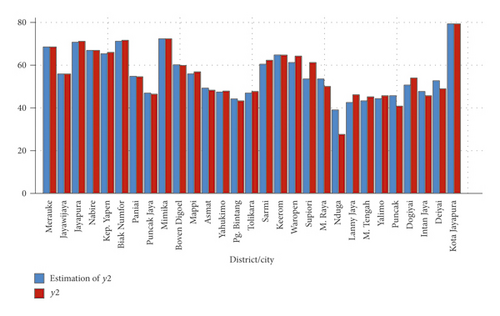
The application of this mixed estimator model on the PPP and HDI in this study is made after the authors conducted a preliminary study. Based on information from the initial research, it is known that the GRDP has a changing pattern at certain subintervals such as the spline pattern. In contrast, the population growth rate has a random pattern that is usually modeled by the kernel. Therefore, the data of PPP and HDI of Papua Province in 2017 are used as response variables, while the predictor variables are the GRDP and the population growth rate. The data were obtained from Statistics Indonesia (Badan Pusat Statistik–BPS), Papua Province, with 29 regencies/cities as the observation unit. The biresponse mixed spline smoothing and kernel estimator in equation (12) was applied to the data. This modeling produces the minimum GCV value of 62.75, the R² of 96.54%, and the RMSE of 3.166. Based on the R² value, it is known that the model can describe the relationship between predictor variables and response up to 96.54%. This finding shows that the biresponse mixed spline smoothing and kernel estimator is suitable for modeling the PPP and HDI in Papua Province. Also, the bar chart in Figures 4 and 5 show that the estimated values of PPP and HDI in Papua Province are close to their actual values.

Furthermore, to determine the predictive ability of this modeling, we use the model that has been obtained from the data in 2017 to predict the PPP and HDI values of Papua Province in 2018 and 2019. This prediction is carried out by applying the model that has been obtained to the GRDP and the population growth rate of Papua Province in 2018 and 2019. One of the criteria for the predictive ability of a model that can be obtained from this prediction is the Mean Absolute Percentage Error (MAPE) value. The MAPE value obtained from the predictions in 2018 is 3.8042% or the level of accuracy is 96.1958%, and the MAPE value from the predictions in 2019 is 5.1658% or the level of accuracy is 94.8342%. These MAPE values are less than 10%, which indicates that the biresponse nonparametric regression model with mixed spline smoothing and kernel estimators has a good predictive ability to predict PPP and HDI in Papua Province.

4. Conclusions

This paper presents the biresponse nonparametric regression model with mixed spline smoothing and kernel estimators. This new mixed estimator is obtained through two-stage estimation, i.e., the first stage using the PWLS to obtain the spline smoothing component, followed by the second stage that employs the WLS to estimate the kernel component. This mixed estimator is formed to handle the different data patterns between each predictor in the biresponse case, so this estimator can provide better estimation results. Selection of the best model for the proposed estimator is carried out by selecting a model that produces a minimum GCV value. The simulation results show the biresponse mixed spline smoothing and kernel estimator provides better results compared to the biresponse spline smoothing or biresponse kernel estimator. Furthermore, this proposed estimator can be appropriately applied to model the percentage of the poor population (PPP) and human development index (HDI) in Papua Province and gives satisfactory results. The limitation of this study is we only use one predictor variable for each component of the estimators, both spline smoothing and kernel estimators. For future work, this biresponse mixed estimator can be developed with more than one predictor for each estimator component. Apart from this limitation, this study is useful for our insight into mixed estimators in biresponse nonparametric regression.

Conflicts of Interest

The authors declare that there are no conflicts of interest in this paper.

Acknowledgments

The authors thank the Ministry of Research, Technology, and Higher Education (Ristekdikti), Republic of Indonesia, for supporting this research through the PMDSU scholarship.

Open Research

Data Availability

The data in this article are available in the BPS of the Papua Province repository (https://papua.bps.go.id).

References

1 Härdle W., Applied Nonparametric Regression, 1990, 19, Cambridge University Press, Cambridge UK.
10.1017/CCOL0521382483
Google Scholar
2 Budiantara I. N., Ratnasari V., Ratna M., Wibowo W. et al., Modeling percentage of poor people in Indonesia using kernel and fourier series mixed estimator in nonparametric regression, Investigacion Operacional. (2019) 40, no. 4, 538–550.
Google Scholar
3 Eubank R. L., Nonparametric Regression and Spline Smoothing, 1999, CRC Press, Boca Raton, FL, USA.
10.1201/9781482273144
Google Scholar
4 Becher H., Kauermann G., Khomski P., and Kouyaté B., Using penalized splines to model age- and season-of-birth-dependent effects of childhood mortality risk factors in rural Burkina Faso, Biometrical Journal. (2009) 51, no. 1, 110–122, https://doi.org/10.1002/bimj.200810496, 2-s2.0-60849100219.
10.1002/bimj.200810496
CAS PubMed Web of Science® Google Scholar
5 Wang Y., Guo W., and Brown M. B., Spline smoothing for bivariate data with applications to association between hormones, Statistica Sinica. (2000) 10, no. 2, 377–397.
Web of Science® Google Scholar
6 Hall P. and Huang L. S., Nonparametric kernel regression subject to monotonicity constraints, Annals of Statistics. (2001) 29, no. 3, 624–647, https://doi.org/10.1214/aos/1009210683, 2-s2.0-0035539846.
10.1214/aos/1009210683
Web of Science® Google Scholar
7 Okumura H. and Naito K., Non-parametric kernel regression for multinomial data, Journal of Multivariate Analysis. (2006) 97, no. 9, 2009–2022, https://doi.org/10.1016/j.jmva.2005.12.008, 2-s2.0-33748437216.
10.1016/j.jmva.2005.12.008
Web of Science® Google Scholar
8 Du P., Parmeter C. F., and Racine J. S., Nonparametric kernel regression with multiple predictors and multiple shape constraints, Statistica Sinica. (2013) 23, no. 3, 1347–1371, https://doi.org/10.5705/ss.2012.024, 2-s2.0-84883879522.
10.5705/ss.2012.024
Web of Science® Google Scholar
9 Chamidah N. and Saifudin T., Estimation of children growth curve based on kernel smoothing in multi-response nonparametric regression, Applied Mathematical Sciences. (2013) 7, no. 37–40, 1839–1847, https://doi.org/10.12988/ams.2013.13168.
10.12988/ams.2013.13168
Google Scholar
10 Erçelik E. and Nadar M., Nonparametric density estimation based on beta prime kernel, Communications in Statistics-Theory and Methods. (2020) 49, no. 2, 325–342, https://doi.org/10.1080/03610926.2018.1538458, 2-s2.0-85057218637.
10.1080/03610926.2018.1538458
Web of Science® Google Scholar
11 Bilodeau M., Fourier smoother and additive models, Canadian Journal of Statistics. (1992) 20, no. 3, 257–269, https://doi.org/10.2307/3315313, 2-s2.0-84988137798.
10.2307/3315313
Web of Science® Google Scholar
12 Amato U., Antoniadis A., and De Feis I., Fourier series approximation of separable models, Journal of Computational and Applied Mathematics. (2002) 146, no. 2, 459–479, https://doi.org/10.1016/S0377-0427(02)00398-9, 2-s2.0-0037106118.
10.1016/S0377-0427(02)00398-9
Web of Science® Google Scholar
13 Hidayat R., Budiantara I. N., Otok B. W., and Ratnasari V., The regression curve estimation by using mixed smoothing spline and kernel (MsS-K) model, Communications in Statistics-Theory and Methods. (2020) 1–12, https://doi.org/10.1080/03610926.2019.1710201.
10.1080/03610926.2019.1710201
Google Scholar
14 Mariati N. P. A. M., Budiantara I. N., and Ratnasari V., Combination estimation of smoothing spline and fourier series in nonparametric regression, Journal of Mathematics. (2020) 2020, 10, https://doi.org/10.1155/2020/4712531, 4712531.
10.1155/2020/4712531
Web of Science® Google Scholar
15 Octavanny M. A. D., Budiantara I. N., Kuswanto H., and Rahmawati D. P., Nonparametric regression model for longitudinal data with mixed truncated spline and fourier series, Abstract and Applied Analysis. (2020) 2020, 11, 4710745, https://doi.org/10.1155/2020/4710745.
10.1155/2020/4710745
Google Scholar
16 Green P. J. and Yandell B. S., Semi-parametric Generalized Linear Models, 1985, Springer, Berlin, Germany, 44–55.
10.1007/978-1-4615-7070-7_6
Google Scholar
17 Roozbeh M. and Arashi M., New ridge regression estimator in semiparametric regression models, Communications in Statistics-Simulation and Computation. (2016) 45, no. 10, 3683–3715, https://doi.org/10.1080/03610918.2014.953685, 2-s2.0-84982915292.
10.1080/03610918.2014.953685
Web of Science® Google Scholar
18 Roozbeh M. and Najarian M., Efficiency of the QR class estimator in semiparametric regression models to combat multicollinearity, Journal of Statistical Computation and Simulation. (2018) 88, no. 9, 1804–1825, https://doi.org/10.1080/00949655.2018.1448088, 2-s2.0-85043698216.
10.1080/00949655.2018.1448088
Web of Science® Google Scholar
19 Akdeniz F. and Roozbeh M., Efficiency of the generalized-difference-based weighted mixed almost unbiased two-parameter estimator in partially linear model, Communications in Statistics-Theory and Methods. (2017) 46, no. 24, 12259–12280, https://doi.org/10.1080/03610926.2017.1295075, 2-s2.0-85028762864.
10.1080/03610926.2017.1295075
Web of Science® Google Scholar
20 Craven P. and Wahba G., Smoothing noisy data with spline functions, Numerische Mathematik. (1978) 31, no. 4, 377–403, https://doi.org/10.1007/BF01404567, 2-s2.0-34250263445.
10.1007/BF01404567
Web of Science® Google Scholar
21 Golub G. H., Heath M., and Wahba G., Generalized cross-validation as a method for choosing a good ridge parameter, Technometrics. (1979) 21, no. 2, 215–223, https://doi.org/10.1080/00401706.1979.10489751, 2-s2.0-32044449925.
10.1080/00401706.1979.10489751
Web of Science® Google Scholar
22 Wahba G., Spline Models for Observational Data, 1990, SIAM, Philadelphia, PA, USA.
10.1137/1.9781611970128
PubMed Google Scholar
23 Amini M. and Roozbeh M., Optimal partial ridge estimation in restricted semiparametric regression models, Journal of Multivariate Analysis. (2015) 136, 26–40, https://doi.org/10.1016/j.jmva.2015.01.005, 2-s2.0-84921947137.
10.1016/j.jmva.2015.01.005
Web of Science® Google Scholar
24 Roozbeh M., Optimal QR-based estimation in partially linear regression models with correlated errors using GCV criterion, Computational Statistics & Data Analysis. (2018) 117, 45–61, https://doi.org/10.1016/j.csda.2017.08.002, 2-s2.0-85028296604.
10.1016/j.csda.2017.08.002
Web of Science® Google Scholar
25 Roozbeh M., Hesamian G., and Akbari M. G., Ridge estimation in semi-parametric regression models under the stochastic restriction and correlated elliptically contoured errors, Journal of Computational and Applied Mathematics. (2020) 378, https://doi.org/10.1016/j.cam.2020.112940.
10.1016/j.cam.2020.112940
Web of Science® Google Scholar
26 Fernandes A. A. R., Budiantara I. N., Otok B. W., and Suhartono L., Spline estimator for bi-responses nonparametric regression model for longitudinal data, Applied Mathematical Sciences. (2014) 8, no. 113–116, 5653–5665, https://doi.org/10.12988/ams.2014.47566, 2-s2.0-84907486155.
10.12988/ams.2014.47566
Google Scholar
27 Madan S., “Human development and poverty–a perspective across Indian states, Statistika. (2012) 49, no. 4, 81–94.
Google Scholar
28 Akhmad A. and Amir S., The effect of economic growth and income inequality on poverty in Indonesia, IOSR Journal of Economics and Finance. (2018) 9, no. 4, 20–26, https://doi.org/10.9790/5933-0904022026.
10.9790/5933-0904022026
Google Scholar
29 Grubaugh S. G., Economic growth and growth in human development, Applied Econometrics and International Development. (2015) 15, no. 2, 5–16.
Google Scholar
30 Mallick S. and Ghani N., A review of the relationship between poverty, population growth and environment, Pakistan Development Review. (2005) 44, no. 4, 597–613, https://doi.org/10.30541/v44i4iipp.597-614.
10.30541/v44i4IIpp.597-614
Google Scholar
31 Sinaga K. P. and Tulus O. D., Analisis Pengaruh Produk Domestik Regional Bruto, Pendidikan dan Pengangguran terhadap Kemiskinan di Kab/Kota Propinsi Sumatera Utara Tahun 2010-2011, Saintia Matematika. (2013) 1, no. 3, 261–271.
Google Scholar
32 Malthus T. R., Review: an essay on the principle of population, Forum for Modern Language Studies. (2005) 41, no. 1, 114–115, https://doi.org/10.1093/fmls/cqi148.
10.1093/fmls/cqi148
Web of Science® Google Scholar
33 Budhi M. K. S., Analisis faktor-faktor yang berpengaruh terhadap pengentasan kemiskinan di bali: analisis FEM data panel, Jurnal Ekonomi Kuantitatif Terapan. (2013) 6, no. 1, 1–70.
Google Scholar

Citing Literature

All articles

Mixed Spline Smoothing and Kernel Estimator in Biresponse Nonparametric Regression

Abstract

1. Introduction

2. Materials and Methods

3. Results and Discussion

3.1. Mixed Spline Smoothing and Kernel Estimator in Biresponse Nonparametric Regression

3.2. Selection of Smoothing and Bandwidth Parameters

3.3. Simulation Study

3.4. Data Application

4. Conclusions

Conflicts of Interest

Acknowledgments

Open Research

Data Availability

References

Citing Literature

Figures

References

Information

About Wiley Online Library

Help & Support

Opportunities

Connect with Wiley

Mixed Spline Smoothing and Kernel Estimator in Biresponse Nonparametric Regression

Abstract

1. Introduction

2. Materials and Methods

3. Results and Discussion

3.1. Mixed Spline Smoothing and Kernel Estimator in Biresponse Nonparametric Regression

3.2. Selection of Smoothing and Bandwidth Parameters

3.3. Simulation Study

3.4. Data Application

4. Conclusions

Conflicts of Interest

Acknowledgments

Open Research

Data Availability

References

Citing Literature

Figures

References

Related

Information