Volume 2021, Issue 1 6088435

Research Article

Open Access

Wood Species Recognition Based on Visible and Near-Infrared Spectral Analysis Using Fuzzy Reasoning and Decision-Level Fusion

Corresponding Author

Peng Zhao

[email protected]

orcid.org/0000-0001-7942-388X

School of Computer Science, Software Engineering and Communication Engineering, Guangxi University of Science and Technology, Liuzhou 545006, China gxut.edu.cn

School of Information and Computer Engineering, Northeast Forestry University, Harbin 150040, China nefu.edu.cn

Search for more papers by this author

Zhen-Yu Li,

Zhen-Yu Li

orcid.org/0000-0001-6941-5982

School of Information and Computer Engineering, Northeast Forestry University, Harbin 150040, China nefu.edu.cn

Search for more papers by this author

Cheng-Kun Wang,

Cheng-Kun Wang

orcid.org/0000-0002-2949-4628

School of Information and Computer Engineering, Northeast Forestry University, Harbin 150040, China nefu.edu.cn

Search for more papers by this author

Peng Zhao,

Corresponding Author

Peng Zhao

[email protected]

orcid.org/0000-0001-7942-388X

School of Computer Science, Software Engineering and Communication Engineering, Guangxi University of Science and Technology, Liuzhou 545006, China gxut.edu.cn

School of Information and Computer Engineering, Northeast Forestry University, Harbin 150040, China nefu.edu.cn

Search for more papers by this author

Zhen-Yu Li,

Zhen-Yu Li

orcid.org/0000-0001-6941-5982

School of Information and Computer Engineering, Northeast Forestry University, Harbin 150040, China nefu.edu.cn

Search for more papers by this author

Cheng-Kun Wang,

Cheng-Kun Wang

orcid.org/0000-0002-2949-4628

School of Information and Computer Engineering, Northeast Forestry University, Harbin 150040, China nefu.edu.cn

Search for more papers by this author

First published: 23 July 2021

https://doi.org/10.1155/2021/6088435

Citations: 5

Academic Editor: Daniel Cozzolino

Share a link

Email
Wechat
Bluesky

Abstract

A novel wood species spectral classification scheme is proposed based on a fuzzy rule classifier. The visible/near-infrared (VIS/NIR) spectral reflectance curve of a wood sample’s cross section was captured using a USB 2000-VIS-NIR spectrometer and a FLAME-NIR spectrometer. First, the wood spectral curve—with spectral bands of 376.64–779.84 nm and 950–1650 nm—was processed using the principal component analysis (PCA) dimension reduction algorithm. The wood spectral data were divided into two datasets, namely, training and testing sets. The training set was used to generate the membership functions and the initial fuzzy rule set, with the fuzzy rule being adjusted to supplement and refine the classification rules to form a perfect fuzzy rule set. Second, a fuzzy classifier was applied to the VIS and NIR bands. An improved decision-level fusion scheme based on the Dempster–Shafer (D-S) evidential theory was proposed to further improve the accuracy of wood species recognition. The test results using the testing set indicated that the overall recognition accuracy (ORA) of our scheme reached 94.76% for 50 wood species, which is superior to that of conventional classification algorithms and recent state-of-the-art wood species classification schemes. This method can rapidly achieve good recognition results, especially using small datasets, owing to its low computational time and space complexity.

1. Introduction

Wood species classification has been investigated for several years, as different wood species have diverse physical and chemical properties. Many such schemes have been proposed for automatic processing using sensors and computers, with spectra-based [1–3], chemometric-based [4], and image-based schemes [5–9] being the most commonly investigated. Spectral analysis technology is also widely used in the prediction of wood properties [10–12] such as wood density [13], wood moisture content [14, 15], and others [16, 17]. The NIR spectral band is often used in these applications. A wood spectral analysis scheme usually pertains to one-dimensional (1D) spectral reflectance curves, which exhibits low computational complexity and, thus, high processing speeds. A wood image processing scheme usually considers the wood’s texture features for species classification, as its texture is more stable than its color [18–20].

Fuzzy logic can provide nonseparated output classes and functions well with just a few learning datasets. In the past, fuzzy-rule-based schemes were successfully used in control systems and pattern recognition applications [21, 22]. In the wood industry, fuzzy rule classification has been successfully applied to wood color classification and wood defect recognition [23–25]. For example, considering the uncertainty of wood color and processing speed, Bombardier et al. proposed a fuzzy rule classifier to fulfill wood color recognition [24, 25].

Fuzzy rule classification is not frequently used in wood species recognition. However, Ibrahim et al. proposed a fuzzy preclassifier to classify 48 tropical wood species into four broad categories, followed by the use of a support vector machine (SVM) classifier in each broad category to further determine the wood species of a sample [19]. One advantage of their approach was that when a new wood species was added to the system, only the SVM classifier of one broad category required retraining instead of the entire system. Similarly, Yusof et al. also proposed a fuzzy-logic-based preclassifier to classify tropical wood species into four broad categories, followed by performing specific wood species recognition using definite classifiers to increase recognition accuracy and decrease processing time requirements [7].

In this study, we propose a fuzzy rule classification scheme for the recognition of 50 wood species using 1D spectral reflectance data. The spectral range covers both the visible (VIS) band (i.e., 376.64–779.84 nm) and the near-infrared (NIR) band (i.e., 950–1650 nm). For the wood spectral curves, the VIS band may vary as the color of a wood sample may change owing to environmental variations, while the NIR band remains relatively stable. Consequently, these two bands were processed using different fuzzy classifiers, and the two classification results were further processed using an improved decision-level fusion based on the D-S evidential theory.

Our scheme has the two following advantages. First, it can achieve good recognition accuracy rapidly in a small spectral dataset. There are only 50 samples for each wood species, and each sample consists of a VIS spectral curve and an NIR curve. Second, the experimental equipment cost is low. The used Ocean Optics USB2000-VIS-NIR spectrometer costs approximately $3,000, while the Ocean Optics FLAME-NIR spectrometer costs $8,000. Several comparisons with other classical and state-of-the-art classifiers in wood species recognition also verified the merits of our scheme.

2. Materials and Methods

2.1. Wood Samples and Spectral Data Acquisition

Our wood dataset consists of 50 wood species, as shown in Table 1 and Figure 1. These 50 wood species consist of softwood and hardwood species, which are representative tree species in the wood market. Moreover, this dataset also consists of some similar wood species (i.e., visually similar wood species and intragenus different species). Each wood sample was processed into a 2 × 2 × 3 cm block. We used the Ocean Optics USB2000-VIS-NIR microfiber spectrometer and an Ocean Optics FLAME-NIR microfiber spectrometer, visible and near-infrared (VIS/NIR) spectra of the wood samples being obtained using these devices. Fifty mean spectral curves were detected by using the spectrometer for each wood species—that is, there are 2500 VIS spectral curves and 2500 NIR spectral curves for 50 wood species. Our experimental setup consisted of a halogen lamp, a universal serial bus, a computer, a customized holder, a fiber spectrometer, and a section of optical fiber, as shown in Figure 2. Spectral acquisition was performed in a controlled environment at a temperature interval of 20 ± 2^°C. The VIS spectral band covered a range of 376.64–779.84 nm, with a spectral resolution of approximately 0.3 nm. The NIR spectral band covered a range of 950–1650 nm, with a spectral resolution of approximately 5.4 nm. The spectrometer parameter settings, spectral data acquisition, and data storage were conducted using the Spectrasuite software. The integration time was 300 ms, and the mean number of measurements at each point was 900. Before spectral acquisition, the reference and dark spectra were measured and stored, the reference spectra were acquired using a standard white panel of known 100% reflectance, and the dark spectra were acquired by blocking the radians. For each wood sample, four diffuse reflectance spectra were measured randomly using (1)—where I_R, I_B, and I_W represented the received intensity, dark intensity, and white panel intensity, respectively—at different locations across the wood sample’s cross section. In fact, wood cross section has plentiful wood structures such as pores and parenchyma, making its spectra more suitable for species recognition, which is superior to radial direction and tangential direction in wood species recognition [26] and wood density prediction [13]. Subsequently, the mean spectrum of each wood sample was calculated and stored for subsequent spectral analysis and species classification. Figures 3 and 4 show the acquired mean spectra of the 50 wood species with standard normal variables (SNVs).

(1)

Table 1. The names of the wood species.

Class label	Latin name
1	Pterocarpus soyauxii
2	Ulmus glabra
3	Calophyllum brasiliense
4	Intsia bijuga
5	Tectona grandis
6	Pouteria speciosa
7	Quercus mongolica
8	Magnolia fordiana
9	Guibourtia ehie
10	Terninalia catappa
11	Cinnamomum camphora
12	Guibourtia demeusei
13	Swintonia florbunda
14	Fraxinus mandshurica
15	Pometia pinnata
16	Dipterocarpus alatus
17	Vernicia fordii
18	Sophora japonica
19	Robinia pseudoacacia
20	Quercus acutissima
21	Populus alba
22	Fraxinus chinensis
23	Pinus sylvestris
24	Populus tomentosa
25	Betula alnoides
26	Betula platyphylla
27	Platanus orientalis
28	Picea asperata
29	Larix gmelinii
30	Salix matsudana
31	Amygdalus davidiana
32	Juglans mandshurica
33	Pinus koraiensis
34	Populus cathayana
35	Tona ciliate
36	Prunus avium
37	Pinus massoniana
38	Aucoumea klaineana
39	Shorea contorta
40	Entandrophragma candollei
41	Millettia laurentii
42	Swietenia mahagoni
43	Rhodamnia dumetorum
44	Cyclobalanopsis glauca
45	Shorea laevis
46	Chamaecyparis nootkatensis
47	Juglans nigra
48	Tilia mandshurica
49	Pseudotsuga menziesii
50	Pinups radiata

Details are in the caption following the image — **Figure 1**
Open in figure viewer PowerPoint

Wood samples for 50 wood species, and the order is the same as that in Table 1 (see Table 1 for specific wood species names).

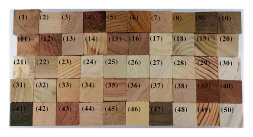
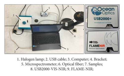
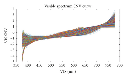
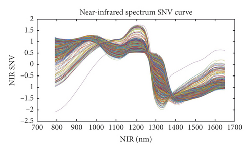
The spectral range of the USB2000-VIS-NIR spectrometer was 340–1027 nm. Both ends of this spectral range can be noisy, so the useful spectral range is 376.64–779.84 nm. The spectral data in the VIS band may be variable as the color of a wood sample may change with changing environmental conditions. To avoid this, we maintained a stable environment during spectral acquisition and wood sample preservation. The NIR band of 950–1650 nm is relatively stable and can be used to characterize different wood properties to some extent. Therefore, these two bands were processed using different fuzzy classifiers—that is, with different membership functions and fuzzy rules—the two classification results of which were further processed using an improved decision-level fusion based on the D-S evidential theory.

2.2. Spectral Dimension Reduction

For each spectral curve, the VIS/NIR band includes thousands of spectral data, so that the spectral dimension is very large. Consequently, each spectral curve contains redundant information, which reduces the wood species classification accuracy and speed. We used principal component analysis (PCA) and the T-distributed stochastic neighbor embedding (T-SNE) algorithms to compare and reduce the spectral dimension results. The PCA algorithm is a transformation algorithm in multivariate statistics, which is based on the variance maximization of a mapped low-dimension vector. The procedure is as follows: First, the initial dataset matrix is defined as A_m×n = [a₁, …, a_n]—where m and n are the dimension and number of feature vectors, respectively. The mean vector is computed as . Second, we compute x_i = a_i − u to form X_m×n = [x₁, …, x_n]. Third, the k largest eigenvalues of XX^T are selected, their k corresponding eigenvectors ε₁, …, ε_k forming a matrix D = [ε₁, …, ε_k]. Finally, the new dataset matrix after dimension reduction is computed as D^T × X = P_k×n(k < m).

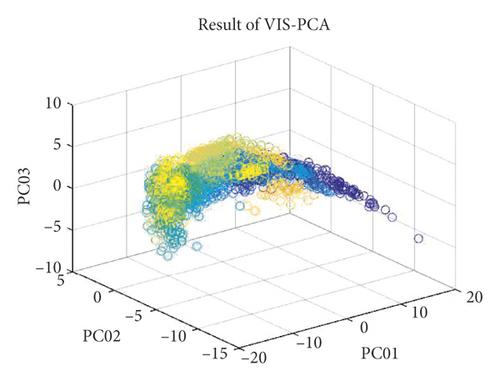
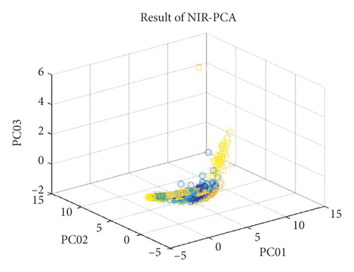
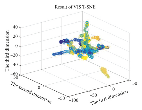
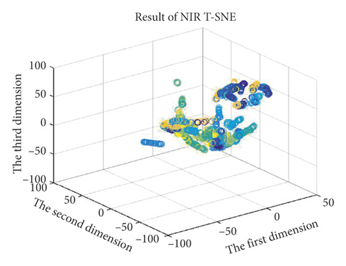
Additionally, the T-SNE algorithm was also used for spectral dimension reduction. This algorithm performs nonlinear dimension reduction, an improvement on the original SNE algorithm [27]. The algorithm is based on the invariant data distribution probability of the mapped low-dimensional vector. Here, the symbol “T” in T-SNE represents the t-distribution, the freedom of the t-distribution being 1 in this study. The graphs of the three-dimensional (3D) spectral vectors for the VIS and NIR bands after spectral dimension reduction using the PCA and T-SNE algorithms are shown in Figure 5. The contribution rate (CR) and cumulative contribution rate (CCR) of the first ten principal components are shown in Figure 6 and Table 2 for the VIS and NIR bands. In Figure 5, the wood sample’s 3D spectral vectors were acquired using the PCA and T-SNE algorithms and are shown with 50 different colors for the 50 wood species. The best case is shown in Figure 5(b), where the wood samples were the most dispersed.

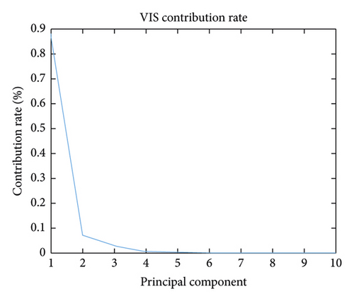
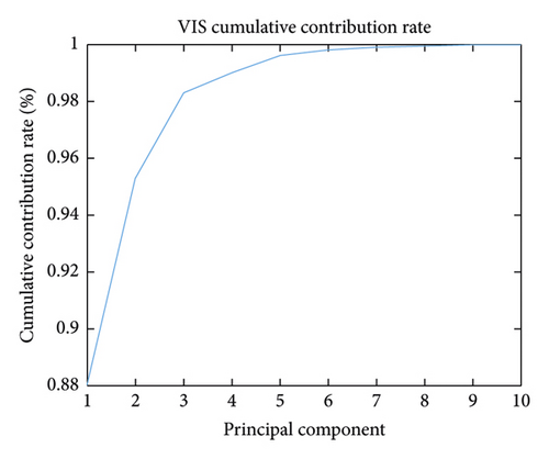
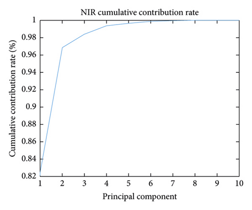
Table 2. The contribution rate (CR) and cumulative contribution rate (CCR) of the principal components (PCs) for visible (VIS) and near-infrared (NIR) spectral data.

	PC01	PC02	PC03	PC04	PC05	PC06	PC07	PC08	PC09	PC10
VIS CR	0.8804	0.0726	0.0301	0.0070	0.0061	0.0018	0.00074982	0.00055908	0.00047882	0.00027888
VIS CCR	0.8804	0.9529	0.9830	0.9900	0.9961	0.9979	0.9986	0.9992	0.9997	0.9999
NIR CR	0.8215	0.1468	0.0155	0.0097	0.0029	0.0021	0.00082330	0.00023093	0.00017311	0.00010637
NIR CCR	0.8215	0.9683	0.9838	0.9935	0.9965	0.9987	0.9994	0.9997	0.9998	0.9999

2.3. Fuzzy Rule Classifier

A fuzzy rule classifier is a fuzzy reasoning system based on fuzzy linguistic rules, its core component being a fuzzy rule set. When an input sample is transformed into the rule set of one wood species, this sample is then classified as a wood species. The overall fuzzy reasoning system is shown in Figure 7 and consists of two parts: the training and testing processes. The steps in Figure 7 are presented as follows.

Step 1. The membership functions are set to fuzzify the training sample’s feature and generate the training sample’s fuzzy rules
Step 2. Fuzzy rules are adjusted by using a corrected confidence coefficient
Step 3. The fuzzy rule set is generated
Step 4. The testing sample’s feature is fuzzified, and the generated rule is compared with the fuzzy rule set for wood species classification

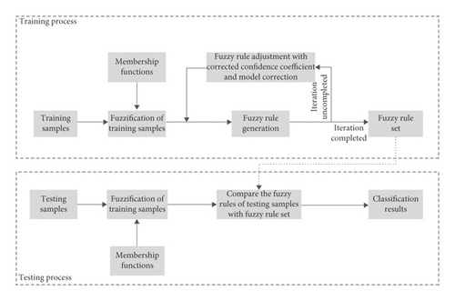
The training process consisted of three steps. First, membership functions were used to fulfill the fuzzification of the training dataset. Here, the membership functions could be a triangular function, trapezoid function, or Gaussian function. Second, fuzzy rules were generated based on the wood species of the wood samples in the training dataset. A fuzzy rule was defined as “IF … AND …, THEN …” using the conjunction or disjunction operation. Third, the fuzzy rules required modification using a confidence coefficient to form a perfect fuzzy rule set.

In the testing process, the testing dataset was added to the trained fuzzy rule classifier, and the same membership functions were used to fulfill its fuzzification. In this way, a corresponding fuzzy rule of a testing sample could be obtained, and this rule was compared with the generated perfect fuzzy rule set to obtain the classified wood species. This species was then compared with the correctly labeled species of the testing sample to evaluate the performance of the fuzzy rule classifier. If the corresponding fuzzy rule of a testing sample was not found in the perfect fuzzy rule set, the sample was classified as an unknown species.

2.3.1. Fuzzification of the Feature Vector

Here, the feature vector refers to the spectral vector after dimension reduction. This fuzzification step transforms spectral feature vectors into linguistic variables. A linguistic variable is defined using a triple value (V, X, T_V), where V is a variable (e.g., PC1) defined on a set of reference X, X is the universe of discourse (field of variation of V), and T_V is the vocabulary chosen to describe the values of V in a symbolic way. The set T_V = {A₁, A₂, …} contains the normalized fuzzy subsets of X, and each fuzzy subset A_i is defined by the membership degree .

For example, the wood spectral feature vector is obtained using the PCA algorithm. The fourth principal component (PC4) of the first ten wood species is shown in Table 3 for the NIR band, where the maximum, minimum, mean, and median values of PC4 are shown. Thus, we can design the membership functions to divide the NIR PC4 (i.e., the 4^th dimension) into twenty-six intervals T_V = {A₁, A₂, …, A₂₆} based on these values, as shown in Figure 8.

Table 3. Principal component 4 (PC4) data for the first ten wood species in the near-infrared (NIR) band.

Wood species	Minimum value	Mean value	Median value	Maximum value
Pterocarpus soyauxii	−0.292834701	−0.16041152	−0.169974712	0.007724295
Ulmus glabra	0.025315788	0.195750566	0.210818609	0.363952969
Calophyllum brasiliense	−0.192778352	−0.117200877	−0.117229875	−0.034786326
Intsia bijuga	−0.389917083	−0.139350711	−0.137772612	0.114471138
Tectona grandis	−0.057557826	0.148158636	0.153314903	0.280022623
Pouteria speciosa	−0.095030985	0.053811088	0.050028547	0.191835329
Quercus mongolica	−0.062964338	0.056146512	0.046516552	0.338022639
Magnolia fordiana	−0.154656742	−0.037434328	−0.048184982	0.126992175
Guibourtia ehie	−0.338868726	−0.178740936	−0.201291866	0.085960311
Terninalia catappa	−0.187178353	0.060716356	0.053703539	0.267102296

As the different spectral PCs or dimensions may be divided into different intervals, the overall number of fuzzy rules is the product of the interval number of different PCs or dimensions:

(2)

where N is the dimension of the spectral feature vectors and Card(T_V) is the number of intervals for variable V (i.e., the element of the spectral feature vector). In fact, N_rules can be determined by both N and Card(T_V). Therefore, a large N or Card(T_V) produces a large N_rules resulting in high computational complexity. In other words, N and Card(T_V) should be designed to be as small as possible in view of the recognition accuracy of our fuzzy rule classifier. If they cannot be simultaneously small, the dimension N should be as small as possible.

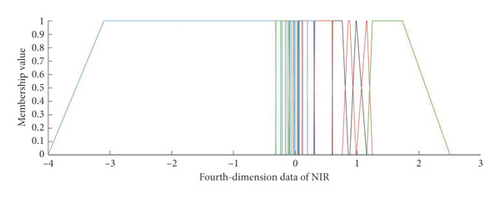
For instance, if the PCA algorithm is used for wood spectral dimension reduction, the CCR should be above 99% in view of the PC number. As can be seen from Table 2, the CCR of the first four PCs reaches 99% and 99.35% for the VIS and NIR bands, respectively, but remains approximately stable when N > 4, so we should set N ≥ 4.

After several tests with the PCA algorithm, N and Card(T_V) were as follows: for the VIS band, Card(T₁) = 37, Card(T₂) = 35, Card(T₃) = 25, Card(T₄) = 21, Card(T₅) = 15, and Card(T₆) = 2. For the NIR band, Card(T₁) = 47, Card(T₂) = 40, Card(T₃) = 28, Card(T₄) = 26, Card(T₅) = 20, and Card(T₆) = 2. The triangular, trapezoid, and triangular-trapezoid functions were used and compared 50 times—in terms of the ORA and mean training time requirement (i.e., the wood sample number of the training set was 2000) for the fuzzy rule set—as described in Tables 4 and 5 for the VIS and NIR bands, respectively. The maximum and practical N_rules in terms of N and Card(T_V) are listed in Table 6. We observed that the training time requirement for the fuzzy rule set was practically invariant with regard to the fuzzy classifiers based on different membership functions. However, this time requirement was only relevant to the N dimension of the spectral feature vectors. In fact, both the time requirement and the N_rules increased rapidly when the dimension N increased. Moreover, the overall recognition accuracy in terms of the triangular-function-based fuzzy classifier increased when the dimension N increased, but the trapezoid-function- or triangular-trapezoid-function-based classifier remained practically invariant when the dimensions were N ≥ 4 and N ≥ 6 for the VIS and NIR bands, respectively. Finally, using our fuzzy classifier, the optimal trapezoid function parameters were dimension N = 37, Card(T₁) = 35, Card(T₂) = 25, Card(T₃) = 25, and Card(T₄) = 21 for the VIS band and N = 4, Card(T₁) = 47, Card(T₂) = 40, Card(T₃) = 28, and Card(T₄) = 26 for the NIR band.

Table 4. Overall recognition accuracy (ORA) and training time requirement (TR) of different N and membership functions in the visible (VIS) band.

Dimension N	Triangular function		Trapezoid function		Triangular-trapezoid
Dimension N	ORA (%)	TR (s)	ORA (%)	TR (s)	ORA (%)	TR (s)
3	75.65	1051.27	76.85	1154.12	77.80	1219.26
4	89.05	24393.24	89.60	25128.75	90.20	24983.20
5	89.60	312764.52	90.05	299023.20	90.25	327279.92
6	90.20	556719.47	90.40	469466.53	90.65	483718.36

Table 5. Overall recognition accuracy (ORA) and training time requirement (TR) of different N and membership functions in the near-infrared (NIR) band.

Dimension N	Triangular function		Trapezoid function		Triangular-trapezoid
Dimension N	ORA (%)	TR (s)	ORA (%)	TR (s)	ORA (%)	TR (s)
3	77.65	1822.23	82.80	1733.46	81.15	1807.12
4	90.25	45125.02	92.90	44783.24	93.25	48353.50
5	91.55	657271.15	93.10	631285.46	92.85	718375.61
6	92.05	1038488.18	93.05	940615.34	93.35	1223481.25

Table 6. Maximum and practical fuzzy rule numbers.

	Dimension N
	3	4	5
(VIS) maximum fuzzy rule number	45325	951825	14277375
(VIS) practical fuzzy rule number	987	1362	1475
(NIR) maximum fuzzy rule number	52640	1368640	27372800
(NIR) practical fuzzy rule number	1135	1674	1689

2.3.2. Fuzzy Rule Generation

After the fuzzification of the spectral feature vectors, the fuzzy rules in the form of “IF … AND …, THEN …” required definition. For example, if three linguistic variables are considered for input (V₁, V₂, V₃) and the output is wood species Y, the fuzzy rule is as follows:

(3)

This expression indicates that when V₁ is classified as A_I, V₂ is classified as B_J …, and the output class is Class_l. Therefore, we need to calculate the membership degrees

for input (V₁, V₂, V₃). In this expression, “AND” is a Cartesian product between the linguistic variables and the operation is performed with a T-Norm, as follows:

(4)

This equation is then used to calculate the product of the membership degrees for the spectral linguistic variables (V₁, V₂, V₃):

(5)

For one wood sample of wood class/species l, there are often some products of the membership degrees

. For example, if

are not equal to 0, we obtain 3 × 2 × 1 = 6 products of the membership degrees for one wood sample (i.e.,

). We should then choose the largest product to form the corresponding rule. Thus, we obtain a fuzzy rule for wood class/species l as follows:

(6)

2.3.3. Fuzzy Rule Adjustment

When the fuzzy rule is generated, there are usually several rules with the same judgment condition (i.e., the same “IF … AND …,”) but different classification results (i.e., different “THEN …”). Consequently, fuzzy rule adjustment is usually required to add a confidence coefficient (CC) to each fuzzy rule.

First, for one wood sample of wood class/species l, the sum of the products of the membership degrees

is calculated as follows:

(7)

Then, the mean value is calculated using

(8)

Thus, we can compute the CC of the fuzzy rule produced as follows:

(9)

Moreover, when the same rules are produced by other samples, the CC of the fuzzy rule should be increased as follows:

(10)

If the same rule is not produced by other samples, the CC of this fuzzy rule remains invariant. Some final rules with their CCs are listed in Table 7. In practical classification work, when there are rules that have the same judgment condition but different classification results, the final classification is determined by the fuzzy rule with the largest CC.

Table 7. The fuzzy rule set with a confidence coefficient (CC) for the visible (VIS) band.

A	B	C	D	CC	Wood species
2	24	8	6	0.9939	Pinups radiata
5	20	9	15	0.9876	Tilia mandshurica
28	29	20	15	0.9072	Juglans nigra
…	…	…	…	…	…
17	2	12	6	0.7993	Entandrophragma candollei
3	23	11	6	0.6161	Chamaecyparis nootkatensis
…	…	…	…	…	…

2.4. Decision-Level Fusion

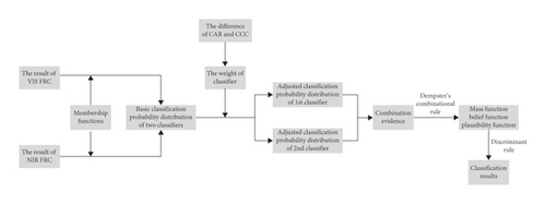
The D-S evidential theory [28] is an effective decision-level fusion scheme, but the classifier’s reliability is not considered fully when each classifier’s result is converted into a classification probability distribution before the decision-level fusion. To solve this problem, we proposed an improved D-S decision-level fusion method that determines each classifier’s weight in view of the differences in the classification accuracy ratio and correlation coefficient.

As the NIR band is more stable than the VIS band, these two bands should be processed using different fuzzy parameters (e.g., different membership functions). Consequently, spectral dimension reduction and fuzzy rule classification were applied to the two bands, respectively, so that the two classification results could be fused with our improved D-S decision-level fusion, as described below. The overall improved D-S decision-level fusion model is shown in Figure 9. The steps in Figure 9 are outlined as follows:

Step 1. The basic classification probability distribution of two classifiers is generated using classification results
Step 2. Classifier weights are determined using classification the accuracy ratio (CAR) and classification correlation coefficient (CCC)
Step 3. The adjusted classification probability distribution is generated using classifier weights
Step 4. The final classification results are calculated using D-S decision-level fusion

2.4.1. Conversion from the Classification Result to Classification Probability Distribution

Based on (4), we calculate the products of membership degrees for the r^VIS dimension of the VIS spectral feature vectors or the r^NIR dimension of the NIR spectral vectors for one wood sample. Every product β_l and its corresponding rule form one row of the matrix Tar:

(11)

where n is the maximum rule number such that n = 951825 for r^VIS = 4 and n = 1368640 for r^NIR = 4.

refers to rule l with product β_l.

Then, the rows with β_l = 0 are deleted in this matrix. The rule

in every row in the matrix Tar is checked to determine whether it belongs to the fuzzy rule set—Table 7—in Section 2.3.3. The rules in the fuzzy rule set remain, while those that are not in the set are deleted in order to form the matrix Tar_pro:

(12)

The added final column Out_nl refers to the corresponding wood species. Some rules in Tar_pro correspond to the same wood species (i.e., Out_ni = Out_nj for i ≠ j). For an Out_nl that corresponds to several rules, the maximum rule (i.e., with the largest β_ni) remains, while the others are deleted, so that the matrix Tar_out is formed. Therefore, for one wood sample, the classification probability distribution can be computed as follows:

(13)

Here, nlast is the number of Tar_out. Note that, for wood species that do not exist in Tar_out, their corresponding classification probabilities are set as 0. For example, the classification probability distribution in the VIS and NIR bands for a wood sample is shown in Table 8.

Table 8. The basic classification probability distribution of the visible/near-infrared (VIS/NIR) fuzzy reasoning classifier (FRC).

Class label	VIS FRC (%)	NIR FRC (%)
1	0.00	0.00
2	0.00	0.00
3	0.00	0.00
4	0.00	0.00
5	0.00	0.00
6	27.22	2.75
7	0.74	0.00
8	0.00	0.00
9	0.00	0.00
10	0.00	0.00
11	0.00	0.00
12	21.45	93.17
13	0.00	0.00
14	1.68	0.00
15	0.00	0.00
16	0.00	0.00
17	14.37	0.00
18	0.00	0.00
19	0.29	0.00
20	0.00	0.00
21	0.00	0.00
22	0.00	0.00
23	0.00	0.07
24	13.15	0.17
25	0.00	0.00
26	0.00	0.00
27	0.00	0.00
28	4.70	0.00
29	0.00	0.62
30	0.00	0.00
31	0.00	0.00
32	0.00	0.00
33	0.00	0.00
34	0.00	0.00
35	0.00	0.00
36	0.00	0.00
37	0.00	2.12
38	0.00	0.00
39	0.00	0.00
40	0.00	0.00
41	3.65	0.00
42	4.32	0.00
43	0.00	0.00
44	0.00	0.35
45	0.00	0.00
46	7.92	0.00
47	0.00	0.00
48	0.00	0.75
49	0.51	0.00
50	0.00	0.00

2.4.2. Weight Determination of VIS and NIR Fuzzy Rule Classifier

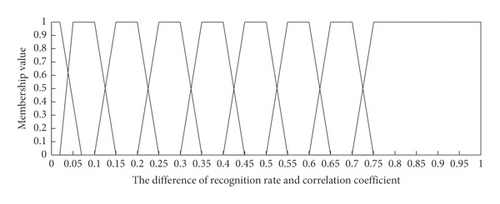
In this section, we propose a novel classifier’s weight determination based on the difference between the fuzzy classification accuracy ratio (CAR) and the correlation coefficient for the VIS and NIR bands using an analytical hierarchy process. In Section 2.3.1, we concluded that the fuzzy classification accuracy was 90.20% after the PCA algorithm processing for r^VIS = 4, while it was 93.25% for r^NIR = 4 in the training set.

Regarding the calculation of the classification correlation coefficient (CCC), the training set is used to calculate the classification probability distribution for each wood sample using (13). Then, the following equation is used to calculate the CCC for the VIS and NIR classifiers:

(14)

Here, Cov(x, y) refers to the covariance between the corrected and actual classification probability distributions. For instance, as described in Table 8, the actual classification probability distribution for one wood sample for the NIR and VIS classifiers was [0,0,0,0,0,2.75, 0, …, 0,0] and [0,0,0,0,0,27.22, 0.74, …, 0.51, 0], respectively, while the corrected one was [0,0,0,0,0,1,0, …, 0]. The σ_x, σ_y represent the standard deviations for the corrected and actual classification probability distribution vectors in the training set, respectively. The computed fuzzy CCC was 0.8073 after PCA algorithm processing for r^VIS = 4, whereas it was 0.8862 for r^NIR = 4.

The difference in the CAR was Diff_CAR = |CAR_VIS − CAR_NIR| = 0.0350, while that of CCC was Diff_CCC = |CCC_VIS − CCC_NIR| = 0.0789. The membership functions are shown in Figure 10. The corresponding credibility for these interval differences is shown in Table 9. We observed that the Diff_CAR was in the 1^st interval, which indicated that the VIS fuzzy and NIR fuzzy classifiers had the same credibility in view of the CAR, while Diff_CCC was in the 2^nd interval, which indicated that the NIR fuzzy classifier was more credible than the VIS classifier in view of the CCC. To determine the classifier’s weight using (17), we first need to compute the classifier’s scores using (15) and then compute the mean score using (16):

(15)

(16)

(17)

Table 9. The relationship between the classification accuracy ratio (CAR) or classification correlation coefficient (CCC) difference interval and its credibility.

RR and CC difference	Credibility	Description
1^st interval	1	The same trusted
2^nd interval	2	Between 1 and 3
3^rd interval	3	A little trusted
4^th interval	4	Between 3 and 5
5^th interval	5	Obviously trusted
6^th interval	6	Between 5 and 7
7^th interval	7	Strongly trusted
8^th interval	8	Between 7 and 9
9^th interval	9	Extremely trusted

2.4.3. Improved D-S Decision-Level Fusion Based on the Classifier’s Weight

In this section, we modified the classification probability distribution, as shown in Table 8, in the VIS and NIR bands using the weight of the classifier. First, the maximum probability was modified using (18), and then, we computed the sum of this modified maximum probability with the other 19 probabilities using (19). Finally, we obtained the modified classification probability distribution using (20). As an example, the classification probability distribution in Table 8 was modified in this manner, as shown in Table 10.

(18)

(19)

(20)

Table 10. The adjustment classification probability distribution of the visible/near-infrared (VIS/NIR) fuzzy reasoning classifier (FRC).

Class label	VIS FRC (%)	NIR FRC (%)
1	0.00	0.00
2	0.00	0.00
3	0.00	0.00
4	0.00	0.00
5	0.00	0.00
6	19.95	2.10
7	0.81	0.00
8	0.00	0.00
9	0.00	0.00
10	0.00	0.00
11	0.00	0.00
12	23.59	94.78
13	0.00	0.00
14	1.85	0.00
15	0.00	0.00
16	0.00	0.00
17	15.81	0.00
18	0.00	0.00
19	0.32	0.00
20	0.00	0.00
21	0.00	0.00
22	0.00	0.00
23	0.00	0.05
24	14.46	0.13
25	0.00	0.00
26	0.00	0.00
27	0.00	0.00
28	5.17	0.00
29	0.00	0.47
30	0.00	0.00
31	0.00	0.00
32	0.00	0.00
33	0.00	0.00
34	0.00	0.00
35	0.00	0.00
36	0.00	0.00
37	0.00	1.62
38	0.00	0.00
39	0.00	0.00
40	0.00	0.00
41	4.01	0.00
42	4.75	0.00
43	0.00	0.00
44	0.00	0.28
45	0.00	0.00
46	8.71	0.00
47	0.00	0.00
48	0.00	0.57
49	0.57	0.00
50	0.00	0.00

Finally, we used the modified VIS and NIR classification probability distributions to compute the normalized constant and composed mass function as follows (i.e.,

(21)

Here, A_i is the i^th wood species with i = 1,2, …, 50. Based on these equations, we can compute 50 mass functions mass(A_i), i = 1,2, …, 50. The first two largest mass(A_i) are defined as mass_max1(A_i), mass_max2(A_i), respectively. mass(f) refers to the mass function for an uncertain set, and in our wood species, the recognition work mass(f) = 0. Wood sample x is then classified as wood species A_j with the following rules: mass(A_j) = mass_max1(A_i), ε₁ = 0.15, ε₂ = 0.01). Otherwise, the judgment is the “rejected classification”:

(22)

3. Results and Comparisons

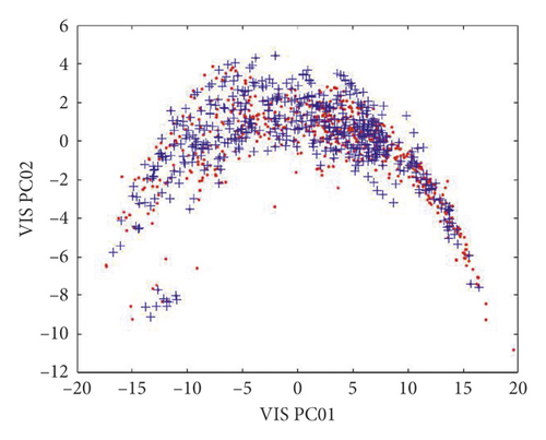
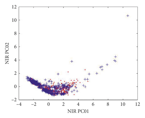
In our experiments, there were 2,500 spectral curves for 50 wood species. These samples were divided into a training set and a testing set using k-fold cross validation [29] with k = 5, so that the training set consisted of 2000 samples and the testing set consisted of 500 samples. Consequently, there were 40 training samples and 10 testing samples for each wood species. The PC1 and PC2 of the training and testing datasets were distributed as shown in Figure 11, where the distributions of both the training and testing sets were dispersed and uniform, indicating that the dataset was suitable for pattern classification.

3.1. Comparisons with Conventional Algorithms

The fuzzy rule classifier was applied to the wood species spectral classification experiments and compared with other important classification schemes, such as the Bayes classifier (BC) [30], random forest (RF) [31], BP network (BPN) [32], SVM [33], and LeNet-5 [34]. The overall recognition accuracy (ORA) and processing speed for a testing sample from our testing dataset (i.e., time requirement, TR) are listed in Table 11. The computer configurations used are presented in Table 12. The ORA was calculated as follows (i.e., n_right is the sample number correctly classified, and n_test is the total sample number of testing sets):

(23)

Table 11. Overall recognition accuracy (ORA) and time requirement (TR) comparisons of the testing dataset for different classifiers (ORA and TR refer to the mean values of 20 tests).

Model	Dataset	ORA (%)	TR (ms)
BC	VIS (PCA7dim)	76.20	0.050256‬
	NIR (PCA7dim)	77.80	0.037920
	VIS (TSNE7dim)	55.00	0.047946
	NIR (TSNE7dim)	61.60	0.052136‬

RF	VIS (PCA7dim)	83.80	2.437714
	NIR (PCA7dim)	84.00	2.326404
	VIS (TSNE7dim)	76.40	2.654658
	NIR (TSNE7dim)	80.40	2.310316

BPN	VIS (PCA7dim)	63.84	0.135030
	NIR (PCA7dim)	61.48	0.117026
	VIS (TSNE7dim)	54.04	0.123924
	NIR (TSNE7dim)	60.80	0.140712

LIBSVM	VIS (PCA7dim)	83.60 (linear)	0.092936
	VIS (PCA7dim)	54.80 (RBF)	0.123525
	NIR (PCA7dim)	84.40 (linear)	0.081890
	NIR (PCA7dim)	80.20 (RBF)	0.131751
	VIS (TSNE7dim)	72.40 (linear)	0.086184
	VIS (TSNE7dim)	23.80 (RBF)	0.253162
	NIR (TSNE7dim)	77.60 (linear)	0.091526
	NIR (TSNE7dim)	23.00 (RBF)	0.211325

LeNet-5	VIS	92.40	0.763721

FRC	VIS (PCA4dim)	90.20	0.137274
	NIR (PCA4dim)	92.92	0.141672
	VIS (TSNE4dim)	71.88	0.159326
	NIR (TSNE4dim)	81.12	0.173528

D-S FRC	VIS + NIR (PCA4dim)	93.84	3.026516
FW-D-S FRC	VIS + NIR (PCA4dim)	94.76	3.071578

VIS: visible band; NIR: near-infrared band; FRC: fuzzy reasoning classifier; PCA: principal component analysis; BC: Bayes classifier; RF: random forest; BPN: BP network; CNN: convolutional neural network; LIBSVM: support vector machine; T-SNE: T-distributed stochastic neighbor embedding; D-S: Dempster–Shafer.

Table 12. The configuration parameters of the computer used.

Configuration	Model	Parameter
CPU	Intel I5-8400	6 core 6 thread, CPU clock speed 2.8 GHz
RAM	Samsung	8 GB, DDR4 2800 MHz
Hard disk	Samsung	256 GB, SSD read: 470 MB/s, write: 473 MB/s

In the RF classification, the time complexity was O(m · n_test · d)—where m is the feature dimension, d is the tree depth, and the RF number is 500. In the BP classification, the time complexity was — where n_i refers to the node number of the i^th layer and d refers to the overall layer number, including the input and output layers. The structure of the BP network was 7 (input layer)-31 (hidden layer)-20 (output layer), and the transfer functions for the input and hidden layers were logsig and purelin, respectively. The BP network’s iteration times were 1000 with a target error and learning rate of 0.01. In the LeNet-5 classification, spectral dimension reduction was not used, whereas the spectral band 451–984 nm was used to form a 40 × 40 matrix. The training dataset was used to train a CNN with a structure comprising six convolution-2 pooling-12 convolution-2 pooling. The size of the convolution cores in the convolutional layers was 5, with a learning rate of 1 and training times of 1000. The time complexity was —where M_i is the size of the output feature image in the i^th layer, K_i is the size of the convolution cores in the i^th convolutional layer, C_i is the core number of the i^th convolutional layer, and d is the overall convolutional layer number. In the SVM classification, a linear kernel function for the PCA algorithm and a radial basis function (RBF) for the T-SNE were used with a penalty factor of 1.2.

In our fuzzy reasoning classifier (FRC) classification, we observed that the PCA algorithm performed much better than the T-SNE algorithm in terms of spectral dimension reduction. The best ORA of 96.3636% was achieved with our FRC, and the D-S decision-level fusion scheme was improved with the use of four PCs for the VIS band and six PCs for the NIR band, with a TR of 2.535915 ms for one testing sample.

In other words, the RF algorithm could achieve good and efficient classification results using a large training dataset. However, its classification performance was poor with our small dataset—our training dataset only consisted of 2000 wood samples—and with low-dimensional feature vectors. Similarly, the BP neural network and LeNet-5 also required a large training dataset to complete network training. Regarding spectral dimension reduction, the classification results using our FRC and T-SNE were relatively poor compared with those of the PCA algorithm as the T-SNE is a nonlinear dimension reduction algorithm.

3.2. Comparisons with State-of-the-Art Algorithms

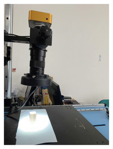
We compared the proposed scheme with other state-of-the-art wood species recognition schemes, all of which performed wood species classification using digital images of wood sample cross sections. We set up the image collection experimental equipment, as shown in Figure 12, consisting of a charge-coupled device (CCD) camera, an optical microscope with a magnification ratio of 10–100, and a light-emitting diode (LED) light source. The wood color image selected was of size 1600 × 1200 pixels and magnification ratio 50. We used this imaging equipment to capture the cross-sectional color image of each wood sample so that each species included 50 images. This color image was then converted into a grayscale image of size 400 × 300 pixels, although the color image was used in the CNN scheme. The computer configuration used is presented in Table 13, and the classification performance comparison is given in Table 14. We found that our FRC and improved D-S decision-level fusion scheme outperformed all other state-of-the-art classification schemes in terms of ORA.

Table 13. Computer configuration parameters.

Configuration	Model	Parameter
CPU	Intel I7–9700F	8 core 8 thread, CPU clock speed 3.00 GHz
GPU	NVIDIA GeForce	8 GB, GDDR6 1650 MHz
GPU	RTX 2060 SUPER	2076 stream processor
RAM	Corsair Memory	16 GB, DDR4 3000 MHZ
Hard disk	Intel	256 GB, SSD read: 1570 MB/s, write 540 MB/s

Table 14. Wood classification performance comparisons with state-of-the-art schemes.

Reference	Model	ORA (%)
[35]	I-BGLAM	72.32
[36]	LBP	68.68
[19, 37]	SPPD	7.32
	SPPD + I-BGLAM	32.68
	Fuzzy + SPPD + BGLAM	34.68
[18]	GA	25.68
[18]	GA + KDA	29.00
[38]	VGG16	83.36
[39]	SqueezeNet	86.28
[40]	ResNet18	94.40
[41]	GoogLeNet	92.80
[42]	CNN	83.00
Our scheme	FRC + improved D-S fusion	94.76

ORA: overall recognition accuracy; TR: time requirement; I-BGLAM: improved basic gray-level aura matrix; LBP: local binary pattern; SPPD: statistical property of pore distribution; GA: genetic algorithm; KDA: kernel discriminant analysis; CNN: convolutional neural network; FRC: fuzzy reasoning classifier; D-S: Dempster–Shafer.

In these state-of-the-art wood species recognition schemes, Yusof et al. employed texture feature operators (e.g., basic gray-level aura matrix (BGLAM), improved basic gray-level aura matrix (I-BGLAM)), and pore distribution features (i.e., statistical properties of pores distribution (SPPD)) and several feature extraction algorithms, such as the genetic algorithm (GA) and kernel discriminant analysis (KDA) to classify more than 50 tropical wood species [18, 19, 35, 37]. However, their schemes were only suitable for the classification of hardwood species with pores. For softwood species without pores, the classification performance of their schemes was poor. Because our 50 wood species consist of both hardwood and softwood species, their schemes delivered poor classification results. Another texture feature operator, the local binary pattern (LBP), and a deep learning neural network were also used for classification comparisons [36, 38–42].

4. Conclusions

In this study, a novel wood species spectral classification scheme was proposed based on a fuzzy linguistic rule classifier and an improved decision-level fusion technique based on the D-S evidential theory. The VIS/NIR spectral reflectance curves of a wood sample’s cross section were measured using a USB 2000-VIS-NIR spectrometer and a FLAME-NIR spectrometer. As the VIS and NIR bands for the wood sample’s cross section have different spectral stabilities, they were processed using two different FRCs, and their classification results were further fused using an improved decision-level fusion technique based on the D-S evidential theory. The test results showed that the best ORA of our scheme reached 94.76% for 50 wood species, with little computational overhead.

More generally, our scheme has the following advantages compared with existing wood species recognition schemes. First, the acquired wood spectral curves were usually noisy and variable because of the variability of the external environment—such as optical illumination intensity—and the wood sample’s internal factors—such as humidity, surface roughness, and intraspecies differences. The uncertainty of these wood spectral features could be resolved using fuzzy processing to some extent. Second, our scheme rapidly achieved good recognition results, particularly with small datasets, and the cost of the VIS/NIR spectrometer used was relatively low. The spectral dataset was a 1D signal set, which had a relatively low computational overhead compared to other 2D image datasets. Therefore, our scheme could be readily applied to wood recognition and classification in the industry in the near future.

However, our scheme can only classify the known wood species which is included in our training dataset. In practical work, some unknown wood species samples may be encountered by our wood classification system. This issue is an unknown species identification problem under the open-world assumption, which can be solved in the certainty or uncertainty framework. For example, in an uncertainty framework, Tang et al. have proposed a new method for generation of generalized basic probability assignment (GBPA) based on evidence theory [43]. In this method, the maximum, minimum, and mean values were used to produce triangular fuzzy number of each class in different attributes, and the intersection points of test samples with triangular fuzzy numbers were calculated. Based on this method, it is feasible to produce a classifier which can effectively recognize the known and unknown classes. Therefore, we plan to investigate and improve this method for wood species classification, since the wood species quantity is greatly larger than the class quantity in [43]. On the other hand, in a certainty framework, we have also used a one-class classifier Support Vector Data Description (SVDD) [44], which can preclassify the wood samples into two categories (i.e., the known and unknown wood categories).

Conflicts of Interest

The authors declare no conflicts of interest.

Acknowledgments

This research was supported by the National Natural Science Foundation of China (Grant no. 31670717) and by the Fundamental Research Funds for the Central University (Grant no. 2572017EB09).

Open Research

Data Availability

Access to research data is restricted. The experimental instruments and wood species samples are owned by other academic institutions; therefore, we cannot publicly release the research spectral and image wood dataset.

References

1 Lavine B. K., Davidson C. E., Moores A. J., and Griffiths P. R., Raman spectroscopy and genetic algorithms for the classification of wood types, Applied Spectroscopy. (2001) 55, no. 8, 960–966, https://doi.org/10.1366/0003702011953108, 2-s2.0-0035414916.
10.1366/0003702011953108
CAS Web of Science® Google Scholar
2 Piuri V. and Scotti F., Design of an automatic wood types classification system by using fluorescence spectra, IEEE Transactions on Systems, Man, and Cybernetics, Part C (Applications and Reviews). (2010) 40, no. 3, 358–366, https://doi.org/10.1109/tsmcc.2009.2039479, 2-s2.0-77951208277.
10.1109/TSMCC.2009.2039479
Web of Science® Google Scholar
3 Moore A. K. and Owen N. L., Infrared spectroscopic studies of solid wood, Applied Spectroscopy Reviews. (2001) 36, no. 1, 65–86, https://doi.org/10.1081/asr-100103090, 2-s2.0-0035244485.
10.1081/ASR-100103090
CAS Web of Science® Google Scholar
4 Miranda I., Gominho J., Ferreira-Dias S., and Pereira H., Pattern recognition as a tool to discriminate softwood and hardwood bark fractions with different particle size, Wood Science and Technology. (2014) 48, no. 6, 1197–1211, https://doi.org/10.1007/s00226-014-0665-9, 2-s2.0-85027949837.
10.1007/s00226-014-0665-9
CAS Web of Science® Google Scholar
5 Khalid M., Eileen L. Y. L., Yusof R. et al., Design of an intelligent wood species recognition system, International Journal of Simulation: Systems, Science and Technology. (2008) 9, no. 3, 9–19.
Google Scholar
6 Khairuddin U., Yusof R., Khalid M. et al., Optimized feature selection for improved tropical wood species recognition system, ICIC Express Letters, Part B. (2011) 2, no. 2, 441–446.
Google Scholar
7 Yusof R., Khalid M., and Mohd Khairuddin A. S., Fuzzy logic-based pre-classifier for tropical wood species recognition system, Machine Vision and Applications. (2013) 24, no. 8, 1589–1604, https://doi.org/10.1007/s00138-013-0526-9, 2-s2.0-84886790583.
10.1007/s00138-013-0526-9
Web of Science® Google Scholar
8 De Geus A. R., Backes A. R., Gontijo A. B. et al., Amazon wood species classification: a comparison between deep learning and pre-designed features, Wood Science and Technology. (2021) 24, https://doi.org/10.1007/s00226-021-01282-w.
10.1007/s00226-021-01282-w
Google Scholar
9 Fabijánska A., Danek M., and Barniak J., Wood species automatic identification from wood core images with a residual convolutional neural network, Computers and Electronics in Agriculture. (2021) 181, 105941.
10.1016/j.compag.2020.105941
Web of Science® Google Scholar
10 Schimleck L. R., Mora C., and Daniels R. F., Estimation of the physical wood properties of green Pinus taeda radial samples by near infrared spectroscopy, Canadian Journal of Forest Research. (2003) 33, no. 12, 2297–2305, https://doi.org/10.1139/x03-173, 2-s2.0-1642282592.
10.1139/x03-173
Web of Science® Google Scholar
11 Popescu M. C., Popescu C. M., Lisa G. et al., Evaluation of morphological and chemical aspects of different wood species by spectroscopy and thermal methods, Journal of Molecular Structure. (2011) 988, no. 1–3, 65–72, https://doi.org/10.1016/j.molstruc.2010.12.004, 2-s2.0-79951673157.
10.1016/j.molstruc.2010.12.004
CAS Web of Science® Google Scholar
12 Schimleck L., Evans R., and Ilic J., Application of near infrared spectroscopy to the extracted wood of a diverse range of species, IAWA Journal. (2003) 24, no. 4, 429–438, https://doi.org/10.1163/22941932-90000347, 2-s2.0-0242658468.
10.1163/22941932-90000347
Web of Science® Google Scholar
13 Jiang Z.-H., Huang A.-M., and Wang B., Near infrared spectroscopy of wood sections and rapid density prediction, Spectroscopy and Spectral Analysis. (2006) 26, no. 6, 1034–1037, in Chinese.
CAS Web of Science® Google Scholar
14 Zhou Z., Rahimi S., Avramidis S. et al., Species- and moisture-based sorting of green timber mix with near infrared spectroscopy, Bioresources. (2020) 15, no. 1, 317–330.
10.15376/biores.15.1.317-330
CAS Web of Science® Google Scholar
15 Tham V. T. H., Inagaki T., and Tsuchikawa S., A new approach based on a combination of capacitance and near-infrared spectroscopy for estimating the moisture content of timber, Wood Science and Technology. (2019) 53, no. 3, 579–599, https://doi.org/10.1007/s00226-019-01077-0, 2-s2.0-85064036798.
10.1007/s00226-019-01077-0
CAS Web of Science® Google Scholar
16 Taylor A. M., Baek S. H., Jeong M. K. et al., Wood shrinkage prediction using NIR spectroscopy, Wood and Fiber Science. (2008) 40, no. 2, 301–307.
CAS Web of Science® Google Scholar
17 Stirling R., Trung T., Breuil C. et al., Predicting wood decay and density using NIR spectroscopy, Wood and Fiber Science. (2007) 39, no. 3, 414–423.
CAS Web of Science® Google Scholar
18 Yusof R., Khalid M., and Khairuddin A. S. M., Application of kernel-genetic algorithm as nonlinear feature selection in tropical wood species recognition system, Computers and Electronics in Agriculture. (2013) 93, no. 1, 68–77, https://doi.org/10.1016/j.compag.2013.01.007, 2-s2.0-84874773345.
10.1016/j.compag.2013.01.007
Web of Science® Google Scholar
19 Ibrahim I., Khairuddin A. S. M., Abu Talip M. S., Arof H., and Yusof R., Tree species recognition system based on macroscopic image analysis, Wood Science and Technology. (2017) 51, no. 2, 431–444, https://doi.org/10.1007/s00226-016-0859-4, 2-s2.0-84988430445.
10.1007/s00226-016-0859-4
CAS Web of Science® Google Scholar
20 Panagiotis B., Kosmas D., Loannis B. et al., Wood species recognition through multidimensional texture analysis, Computers and Electronics in Agriculture. (2018) 144, no. 2, 241–248, https://doi.org/10.1016/s0168-1699(17)31597-1.
10.1016/j.compag.2017.12.011
Web of Science® Google Scholar
21 Roubos J. A., Setnes M., and Abonyi J., Learning fuzzy classification rules from labeled data, Information Sciences. (2003) 150, no. 1-2, 77–93, https://doi.org/10.1016/s0020-0255(02)00369-9, 2-s2.0-0037361892.
10.1016/S0020-0255(02)00369-9
Web of Science® Google Scholar
22 Nakashima T., Schaefer G., Yokota Y., and Ishibuchi H., A weighted fuzzy classifier and its application to image processing tasks, Fuzzy Sets and Systems. (2007) 158, no. 3, 284–294, https://doi.org/10.1016/j.fss.2006.10.011, 2-s2.0-33845212542.
10.1016/j.fss.2006.10.011
Web of Science® Google Scholar
23 Bombardier V., Mazaud C., Lhoste P., and Vogrig R., Contribution of fuzzy reasoning method to knowledge integration in a defect recognition system, Computers in Industry. (2007) 58, no. 4, 355–366, https://doi.org/10.1016/j.compind.2006.07.006, 2-s2.0-33947317868.
10.1016/j.compind.2006.07.006
Web of Science® Google Scholar
24 Bombardier V., Schmitt E., and Charpentier P., A fuzzy sensor for color matching vision system, Measurement. (2009) 42, no. 2, 189–201, https://doi.org/10.1016/j.measurement.2008.05.007, 2-s2.0-57649111438.
10.1016/j.measurement.2008.05.007
Web of Science® Google Scholar
25 Bombardier V. and Schmitt E., Fuzzy rule classifier: capability for generalization in wood color recognition, Engineering Applications of Artificial Intelligence. (2010) 23, no. 6, 978–988, https://doi.org/10.1016/j.engappai.2010.05.001, 2-s2.0-77953962613.
10.1016/j.engappai.2010.05.001
Web of Science® Google Scholar
26 Barmpoutis P., Dimitropoulos K., Barboutis I., Grammalidis N., and Lefakis P., Wood species recognition through multidimensional texture analysis, Computers and Electronics in Agriculture. (2018) 144, 241–248, https://doi.org/10.1016/j.compag.2017.12.011, 2-s2.0-85037973604.
10.1016/j.compag.2017.12.011
Web of Science® Google Scholar
27 Maaten L. V. D. and Hinton G., Visualizing data using t-SNE, Journal of Machine Learning Research. (2008) 9, 2579–2605.
Web of Science® Google Scholar
28 Smets P., The combination of evidence in the transferable belief model, IEEE Transactions on Pattern Analysis and Machine Intelligence. (1990) 12, no. 5, 447–458, https://doi.org/10.1109/34.55104, 2-s2.0-0025434991.
10.1109/34.55104
Web of Science® Google Scholar
29 Bengio Y. and Grandvalet Y., No unbiased estimator the variance of K-fold cross-validation, Journal of Machine Learning Research. (2004) 5, 1089–1105.
Web of Science® Google Scholar
30 Lewis D. D., Naive (Bayes) at forty: the independence assumption in information retrieval, Lecture Notes in Computer Science European Conference on Machine Learning. (1998) 1398, 4–15.
10.1007/BFb0026666
Google Scholar
31 Belgiu M. and Drăguţ L., Random forest in remote sensing: a review of applications and future directions, ISPRS Journal of Photogrammetry and Remote Sensing. (2016) 114, no. 4, 24–31, https://doi.org/10.1016/j.isprsjprs.2016.01.011, 2-s2.0-84961834117.
10.1016/j.isprsjprs.2016.01.011
Web of Science® Google Scholar
32 Zipser D. and Andersen R. A., A back-propagation programmed network that simulates response properties of a subset of posterior parietal neurons, Nature. (1988) 331, no. 6158, 679–684, https://doi.org/10.1038/331679a0, 2-s2.0-0023877474.
10.1038/331679a0
CAS PubMed Web of Science® Google Scholar
33 Chang C.-C. and Lin C.-J., Libsvm, ACM Transactions on Intelligent Systems and Technology. (2011) 2, no. 3, 1–27, https://doi.org/10.1145/1961189.1961199, 2-s2.0-79955702502.
10.1145/1961189.1961199
Web of Science® Google Scholar
34 Lecun Y., Bottou L., Bengio Y., and Haffner P., Gradient-based learning applied to document recognition, Proceedings of the IEEE. (1998) 86, no. 11, 2278–2324, https://doi.org/10.1109/5.726791, 2-s2.0-0032203257.
10.1109/5.726791
Web of Science® Google Scholar
35 Zamri M. I. A. P., Cordova F., Khairuddin A. S. M., Mokhtar N., and Yusof R., Tree species classification based on image analysis using improved-basic gray level aura matrix, Computers and Electronics in Agriculture. (2016) 124, 227–233, https://doi.org/10.1016/j.compag.2016.04.004, 2-s2.0-84963796119.
10.1016/j.compag.2016.04.004
Web of Science® Google Scholar
36 Ojala T., Pietikäinen M., and Mäenpää T., Multiresolution gray-scale and rotation invariant texture classification with local binary patterns, IEEE Transactions on Pattern Analysis and Machine Intelligence. (2002) 24, no. 7, 971–987, https://doi.org/10.1109/tpami.2002.1017623, 2-s2.0-0036647193.
10.1109/TPAMI.2002.1017623
Web of Science® Google Scholar
37 Ibrahim I., Khairuddin A. S. M., Arof H., Yusof R., and Hanafi E., Statistical feature extraction method for wood species recognition system, European Journal of Wood and Wood Products. (2018) 76, no. 1, 345–356, https://doi.org/10.1007/s00107-017-1163-1, 2-s2.0-85015843179.
10.1007/s00107-017-1163-1
Web of Science® Google Scholar
38 Simonyan K. and Zisserman A., Very deep convolutional networks for large-scale image recognition, 2014, https://arxiv.org/abs/1409.1556.
Google Scholar
39 Iandola F. N., Han S., Moskewicz M. W. et al., SqueezeNet: AlexNet-level accuracy with 50x fewer parameters and <0.5 MB model size, 2016, https://arxiv.org/abs/1602.07360.
Google Scholar
40 He K., Zhang X., Ren S., and Sun J., Deep residual learning for image recognition, Proceedings of the IEEE Conference on Computer Vision and Pattern Recognition (CVPR), June 2016, Las Vegas, NV, USA, 770–778, https://doi.org/10.1109/CVPR.2016.90, 2-s2.0-84986274465.
10.1109/CVPR.2016.90
Google Scholar
41 Szegedy C., Wei Liu W., Yangqing Jia Y. et al., Going deeper with convolutions, Proceedings of the IEEE Conference on Computer Vision and Pattern Recognition (CVPR), June 2015, Boston, MA, USA, 1–9, https://doi.org/10.1109/CVPR.2015.7298594, 2-s2.0-84937522268.
10.1109/CVPR.2015.7298594
Google Scholar
42 Oktaria A. S., Prakasa E., and Suhartono E., Wood species identification using convolutional neural network (CNN) architectures on macroscopic images, Journal of Information Technology and Computer Science. (2019) 4, no. 3, 274–283, https://doi.org/10.25126/jitecs.201943155.
10.25126/jitecs.201943155
Google Scholar
43 Tang Y., Wu D., and Liu Z., A new approach for generation of generalized basic probability assignment in the evidence theory, Pattern Analysis and Applications. (2021) https://doi.org/10.1007/s10044-021-00966-0.
10.1007/s10044-021-00966-0
Web of Science® Google Scholar
44 Zhao P., Li Z.-Y., and Li Y., An incremental self-adaptive wood species classification prototype system, Journal of Spectroscopy. (2019) 2019, 11, 9247386, https://doi.org/10.1155/2019/9247386.
10.1155/2019/9247386
Web of Science® Google Scholar

Citing Literature

All articles

Wood Species Recognition Based on Visible and Near-Infrared Spectral Analysis Using Fuzzy Reasoning and Decision-Level Fusion

Abstract

1. Introduction

2. Materials and Methods