In this study, the spreading of the pandemic coronavirus disease (COVID-19) is formulated mathematically. The objective of this study is to stop or slow the spread of COVID-19. In fact, to stop the spread of COVID-19, the vaccine of the disease is needed. However, in the absence of the vaccine, people must have to obey curfew and social distancing and follow the media alert coverage rule. In order to maintain these alternative factors, we must obey the modeling rule. Therefore, the impact of curfew, media alert coverage, and social distance between the individuals on the outbreak of disease is considered. Five ordinary differential equations of the first-order are used to represent the model. The solution properties of the system are discussed. The equilibria and the basic reproduction number are computed. The local and global stabilities are studied. The occurrence of local bifurcation near the disease-free equilibrium point is investigated. Numerical simulation is carried out in applying the model to the sample of the Iraqi population through solving the model using the Runge–Kutta fourth-order method with the help of Matlab. It is observed that the complete application of the curfew and social distance makes the basic reproduction number less than one and hence prevents the outbreak of disease. However, increasing the media alert coverage does not prevent the outbreak of disease completely, instead of that it reduces the spread, which means the disease is under control, by reducing the basic reproduction number and making it an approachable one.

1. Introduction

The most considerable species in habitat are viruses. Since they cannot reproduce themselves, they are known as parasites. Some of these viruses, when they are replicated, cause dangerous diseases in the host, whether humans or animals. One of these species is the coronavirus (COVID-19). It is a disease caused by a new coronavirus called SARS-CoV-2. An outbreak of pneumonia caused by a novel coronavirus (COVID-19) began on 31 December 2019, in Wuhan, China. This pandemic that rapidly spread over 215 countries as of March 2020 continues to hit heavy public health and socio-economic burden in many parts of the world, including in Iraq. From January 22, 2020, up to March 3, 2021, it was reported that over 115 million confirmed cases and about 2,565,310 deaths around the world [1].

The experience in China showed that the use of complete curfew and the speed diagnosis of the infected individuals have a strong impact on the dynamics of the epidemic [2]. It is well known that there is a long history of applying mathematical models in epidemiology to understand and control the outbreak of disease. Carcione et al. [3] implemented an SEIR model to compute the COVID-19 infected population and the number of casualties of this epidemic. Eikenberry et al. [4] developed a compartmental model for assessing the community-wide impact of masks used in the US states of New York and Washington by the general, asymptomatic public, a portion of which may be asymptomatically infectious. Maji [5] formulated a mathematical model for the COVID-19 outbreak by introducing a quarantine class with media-induced fear in the disease transmission rate to analyze the dynamic behavior of this epidemic. Asamoah et al. [6] developed a deterministic model to study the transmission dynamics of the disease with two categories of the susceptibles: Immigrant Susceptibles and Local Susceptible. Peter et al. [7], proposed a new mathematical model to investigate the recent outbreak of coronavirus disease (COVID-19) in Pakistan. Das et al. [8] formulated a mathematical model with comorbidity to study the transmission dynamics as well as an optimal control-based framework to diminish COVID-19. Musa et al. [9] employed an SEIR model to study the transmission dynamics of SARS-CoV-2 outbreaks in Nigeria; the model incorporates a different group of populations, namely, high and moderate risk populations. They used the model to investigate the influence of each population on the overall transmission dynamics. Recently, Paul et al. [10] proposed a simple population dynamics solution based on the incidence-fitness relationship in predicting that a plateau or steady-state of SARS-CoV-2 will be reached using the basic concept of geometry. Many other researchers have been proposed and studied mathematical models to describe the dynamic of COVID-19 (see [11–14] and the references therein).

In view of the above, in this paper, however, a mathematical model that describes the spreading of COVID-19 is proposed and studied. It is assumed that the population is divided into five compartments including susceptible, exposed, infected, hospitalized infected, and recovered. The impact of curfew, media alert coverage, and social distance on the dynamical behavior of the model is considered. The paper is organized as follows. Section 2 treats the formulation of the model with standard properties of the solution of the model. Section 3 interests in the existence of equilibria and computing the basic reproduction number. Section 4 studies local stability. While global stability is discussed in Section 5. The local bifurcation analysis is investigated in Section 6. However, Section 7 contained the numerical simulation for the model. Finally, Section 8 gives the discussion and conclusion of this study.

2. Formulation of the Model

In this section, the dynamics of COVID-19 are mathematically modeled using first-order ordinary differential equations. It is known that COVID-19 is transmitted mainly from humans to humans through direct contact between them. Accordingly, the population is divided into a number of separated compartments depending on the rules of the health section. Therefore, the population can be divided into five main compartments; these are the susceptible individuals at time t denoted by S(t) in which the individuals are at risk of infection with COVID-19. The exposed individuals at time t are denoted by E(t), in which the individuals have contracted the COVID-19 but are not yet infectious. The infected individuals at time t are represented as I(t) in which the individuals are capable of spreading the disease, and they are having mild symptoms or not. The hospitalized infected individuals at time t are denoted by I_h(t), in which the individuals have severe symptoms or quarantined due to getting mild symptoms, and they put in the hospital to get treatment. Finally, the recovered individuals at time t are denoted by R(t) in which the individuals have recovered from the disease and are no more infectious. Therefore, the mathematical model that describes the dynamics of COVID-19 can be described as follows:

()

All the parameters are nonnegative real numbers, and their descriptions are explained in Table 1. Note that b(I) = (b₁ − b₂I/m + I) is the contact rate after the media alert (see [15]). The choice of this function to describe the media alert is due to the following reasons. Most human beings will protect themselves from infection using all possible ways as soon as infected individuals are reported by media coverage. This reduces the transmission rate more or less. Accordingly, as the infected individuals increase, the susceptible individuals reduce their contact with other individuals to avoid the infection. Moreover, the term (b₂I/m + I) refers to the reduced value of the contact (transmission) rate in the case of reporting of the infectious individuals. Clearly, as the infected individuals increase without bound, the term (b₂I/m + I) approaches its maximum that is given by b₂. However, the value of (b₂I/m + I) equals half of the maximum b₂ when the reported infective number arrives at m. Finally, since the media alert report cannot prevent the disease from spreading completely, it is assumed that b₁ ≥ b₂.

Table 1. The parameters description.

Parameter	Description
A	The recruitment rate
c	The probability of individuals responding to the curfew
b₁	The direct contact rate between S and I in the absence of media alerts
b₂	The direct contact rate between S and I in the existence of media alerts
m	Nonresponse rate of the individuals to the media alerts
p	The rate of incubation termination and transition from uninfected to infectious individuals
q	The fraction of the exposed individuals move to the infected compartment, while the rest (1 − q) moves to the hospitalized infected population
r₁	The recovery rate due to natural immune response
r₂	The recovery rate due to treatment
v	The fraction of the nonrecovered individuals who start suffering severe symptoms move to the hospitalized infected population
d₀	The natural death rate
d₁	The death rate of disease in the infectious compartment
d₂	The death rate due to disease in the hospitalized infected population

Recall that the interaction functions between the compartments given by the right-hand side of the system (1) are continuous and have continuous partial derivatives. Therefore, they are Lipschitz functions, and hence system (1) has a unique solution.

Theorem 1. All solutions of system (1) which initiate in are uniformly bounded.

Proof. Let (S(t), E(t), I(t), I_h(t), R(t)) be any solution of system (1) that initiates at the nonnegative value (S(0), E(0), I(0), I_h(0), R(0)).

Consider the function N(t) = S(t) + E(t) + I(t) + I_h(t) + R(t).

By taking the derivative of N(t) with respect to the time along with the solution of system (1), it is obtained that

()

Then, using direct computation gives that

()

Accordingly, it is obtained that

()

which implies that N(t) ≤ A/d₀, as t⟶∞. Hence, all the solutions of system (1) are uniformly bounded, and therefore we finished the proof.

According to system (1), the feasible region of it can be written as follows:

()

3. Existence of the Equilibrium Points and Basic Reproduction Number

Note that since the variable R, which represents the recovered individuals, dose not appear in the first four equations of system (1), hence one can solve the following system instead of system (1) and then substitute the solution values of I and I_h in the fifth equation of system (1) to solve it separately as a linear differential equation with respect to the variable R. Straightforward computation gives that the solution of the fifth equation as t⟶∞ can be written as

()

where

represents the solution values of system (7).

Accordingly, the following system will be studied instead of system (1):

()

Clearly, system (7) has two equilibrium points: the disease-free equilibrium point and the endemic equilibrium point. The disease-free equilibrium point is given by ρ₀ = (S₀, 0,0,0), where

()

Since the basic reproduction number is computed at this equilibrium point, hence in the following the computation of this number is carried out, and then the endemic equilibrium point is determined.

Now, in order to determine the basic reproduction number, the “next-generation method” or “Spectral Radius method” is used (see [16, 17]). Consider an epidemic model having n different compartments from which m compartments contained infected individuals with the disease, then the next-generation matrix (operator) is given by (FV)⁻¹, where

()

where i, j = 1,2, …, m, ρ₀ is the disease-free equilibrium point, while x_i denotes the number of individuals in the i^th infected compartment. However, F_i(x_i) is the rate of appearance of new infections in the compartment i, while

where

represents the rate of the shift of individuals into i^th compartment by all other means and

denotes the rate of the shift of individuals out of the i^th compartment. The difference F_i(x_i) − V_i(x_i) gives the rate of change of x_i. Note that F_i should include only infections that are newly arising but does not include terms that describe the shift of infectious individuals from one infected compartment to another. Finally, the basic reproduction number, that is denoted by R₀, is given by the spectral radius (dominant eigenvalue) of the matrix FV⁻¹. It is well known that the basic reproduction number R₀ is one of the most crucial quantities in infectious diseases as R₀ measures how contagious a disease is. For R₀ < 1, the disease is expected to stop spreading, but for R₀ = 1, an infected individual can infect on an average 1 person; that is, the spread of the disease is stable. The disease can spread and become epidemic if R₀ > 1.

Accordingly, regarding system (7), it is obtained that

()

where B₁ = p + d₀, B₂ = r₁ + v(1 − r₁) + (d₀ + d₁), and B₃ = r₂ + (d₀ + d₂). Then, we get

()

Therefore,

()

Consequently, the basic reproduction number of system (7) is determined as

()

Now, the endemic equilibrium point of system (7) can be determined by

, where

()

where B₄ = r₁ + d₀ + d₁, while E^∗ is a positive root of the second-order polynomial equation:

()

where α₁ = −(1 − c)(b₁–b₂)B₁(qp)² < 0, α₂ = qp[(1 − c)(b₁–b₂)Aqp − (1 − c)b₁mB₁B₂ − B₁B₂], and α₃ = mB₂[(1 − c)b₁qpA − B₁B₂d₀] = B₁B₂d₀mB₂[R₀ − 1].

Therefore, equation (11) has a unique positive root, given by

, if and only if the following condition holds:

()

Moreover, in order to obtain a positive endemic equilibrium point ρ₁ for system (7), we should have

()

4. Local Stability Analysis

This section treats the local stability of system (7) using the linearization technique. The Jacobian matrix for system (7) at the point (S, E, I, I_h) can be written as follows:

()

where the symbols B_i, i = 1,2,3, are given in equation (10). Therefore, the local stability analysis for the disease-free equilibrium point can be studied in the following theorem.

Theorem 2. The disease-free equilibrium point (ρ₀) of system (7) is locally asymptotically stable provided the following condition holds:

()

Proof. According to equation (18), the Jacobian matrix at the point (ρ₀) is given by

()

Direct computations show that this Jacobian matrix has the following characteristic equation:

()

where T = −(B₁ + B₂) < 0 and D = B₁B₂ − (1 − c)qpb₁S₀ = B₁B₂[1 − R₀]. Therefore, all the eigenvalues of the matrix J(ρ₀) are real and negative if and only if condition (19) holds. Moreover, since the other two eigenvalues λ₁ = −d₀ and λ₄ = −B₃ are negative, hence the disease-free equilibrium point (ρ₀) of system (7) is locally asymptotically stable under condition (19). However, if condition (19) is revised, then ρ₀ is an unstable point. Thus, this completes the proof.

According to theorem (6), the basic reproduction number represents the vital value for controlling the outbreak of COVID-19, so that the disease will disappear provided that the basic reproduction number is less than one while the COVID-19 will outbreak when the basic reproduction number is greater than one.

Theorem 3. The endemic equilibrium point (ρ₁) of system (7) is locally asymptotically stable provided that

()

where b_ij, i, j = 1,2,3, are given in the proof.

Proof. Substituting the endemic equilibrium point (ρ₁) in the Jacobian matrix given by equation (18) gives that

()

where b₁₁ = −(1 − c)(b₁–b₂I^∗/m + I^∗)I^∗ − d₀,

, b₂₁ = (1 − c)(b₁–b₂I^∗/m + I^∗)I^∗, b₂₂ = −B₁,

, b₃₂ = qp, b₃₃ = −B₂, b₄₂ = (1 − q)p, b₄₃ = v(1 − r₁), and b₄₄ = −B₃.

Hence, the characteristic equation of this Jacobian matrix can be written as

()

where A₁ = −[b₁₁ + b₂₂ + b₃₃], A₂ = b₁₁b₂₂ + b₁₁b₃₃ + b₂₂b₃₃–b₂₃b₃₂, and A₃ = −[b₁₁b₂₂b₃₃ + b₁₃b₂₁b₃₂ − b₁₁b₂₃b₃₂].

While Δ = A₁A₂ − A₃ = A₁[b₁₁b₂₂ + b₂₂b₃₃ − b₂₃b₃₂] − b₁₁b₃₃(b₁₁ + b₃₃), accordingly, by substituting the values of b_ij and then using condition (22) along with the existence condition (16), we obtain that A₁, A₃, and Δ are positive. Therefore, all the roots (eigenvalues) of the third-order polynomial equation in (24) have negative real parts. Furthermore, since the fourth eigenvalue λ₄ = b₄₄ = −B₃ < 0, then the proof is complete.

From theorem (7), it concluded that the COVID-19 will be endemic and the disease is out of control if in addition to the basic reproduction number greater than one, condition (22) is satisfied.

5. Global Stability

In this section, the stability analysis of system (7) is studied using the Lyapunov function in order to obtain the global stability conditions or the basin of attraction for each equilibrium point. Therefore, the following theorem discusses the global stability of the free-disease equilibrium point.

Theorem 4. Assume that free-disease equilibrium point ρ₀ = (A/d₀, 0,0,0) is locally asymptotically stable, then it is global asymptotically stable.

Proof. Consider the following positive definite real valued function:

()

Clearly, , V₀(ρ₀) = 0, and V₀(x) > 0 where x ≠ ρ₀. Moreover, direct computation gives that

()

Clearly, we have dV₀/dt ≤ 0 if and only if the local stability condition (19) for the free-disease equilibrium point holds. Hence, V₀ is negative definite for any initial point that belongs to , and then the proof is complete.

Theorem 5. Assume that endemic equilibrium point is locally asymptotically stable, then it is a global asymptotically stable provided that the following conditions hold:

()

where all the symbols π_ij are given in the proof.

Proof. Consider the positive definite function

()

Clearly, , V₁(ρ₁) = 0, and V₁(x) > 0 where x ≠ ρ₁. Moreover, direct computation gives that

()

where π₁₁ = d₀ + (1 − c)I^∗/(m + I)(m + I^∗)[mb₁(1 + I) + (b₁ − b₂)(m + I)I^∗], π₁₂ = (1 − c)I^∗/(m + I)(m + I^∗)[mb₁(1 + I) + (b₁ − b₂)(m + I)I^∗], π₁₃ = (1 − c)S/(m + I)(m + I^∗)[m[b₁ + (b₁ − b₂)I] + (b₁ − b₂)(m + I)I^∗], π₂₃ = (1 − c)S/(m + I)(m + I^∗)[m[b₁ + (b₁ − b₂)I] + (b₁ − b₂)(m + I)I^∗] + qp, and π₂₄ = (1 − q)p, π₃₄ = v(1 − r₁).

Accordingly, by using conditions (27a)–(27e), we obtain that

()

Clearly, the derivative dV₁/dt is negative definite for any initial point belonging to , and then the proof is complete.

6. The Local Bifurcation Analysis

Rewrite system (7) in the form as follows:

()

where the functions f_i, i = 1,2,3,4, are the interaction functions given on the right-hand side of system (7). Accordingly, the second derivative of F with respect to X can be written as

()

where

be any nonzero vector. Therefore, the local bifurcation condition at the disease-free equilibrium point is established by the following theorem.

Theorem 6. System (7) exhibits a transcritical bifurcation near the disease-free equilibrium point ρ₀, where R₀ = 1 or .

Proof. Straightforward computation shows that the Jacobian matrix of system (7) at (ρ₀, b₁ ^∗) can be written as

()

Therefore, the eigenvalues of J₀ can be written as

()

Accordingly, the disease-free equilibrium point becomes the nonhyperbolic point. Now, define as the eigenvector corresponding to the eigenvalue λ₀₃ = 0. Direct computation gives that

()

where η₁ = −B₁B₂/qpd₀ < 0, η₂ = B₂/qp > 0, and η₃ = 1/B₃[(1 − q)B₂/q + v(1 − r₁)] > 0, with x₃ be any nonzero real number.

()

where η₄ = qp/B₁ > 0, with y₃ be any nonzero real number.

Define as the eigenvector corresponding to the eigenvalue λ₀₃ = 0 of the matrix . Direct computation gives that

Hence,

()

Then, it is obtained that . Furthermore, it is observed that

()

Therefore, . However, substituting the values of U₁ in equation (32) instead of V and then computing give that

()

Clearly, . Hence, all the transcritical bifurcation conditions in the sense of Sotomayor’s theorem are satisfied. Therefore, the proof is complete.

It is observed that although system (7) becomes a nonhyperbolic near the endemic equilibrium point ρ₁ as p = −b₁₁b₂₂b₃₃/q(b₁₃b₂₁ − b₁₁b₂₃)(≡p^∗) where b_ij, ij = 1,2,3,4 are the elements if J(ρ₁) that is given in equation (23), it does not exhibit any types of local bifurcation in the sense of Sotomayor. This is can be verified directly by substituting the values of ρ₁ and p^∗ in the value of A₃ that is given in equation (24) and then computing the eigenvectors corresponding to the resulting zero eigenvalues of J(ρ₁, p^∗) and their transpose, respectively.

It is obtained that the eigenvectors corresponding to the zero eigenvalue of J(ρ₁, p^∗) and their transpose are, respectively, given by

()

where μ₁ = −ξ₂/(ξ₁ + d₀) < 0, μ₂ = ξ₂d₀/(ξ₁ + d₀)(p^∗ + d₀) > 0, and μ₃ = 1/B₃[(1 − q)p^∗ξ₂d₀/(ξ₁ + d₀)(p^∗ + d₀) + v(1 − r₁)] > 0, with z₃ and w₃ are any nonzero real numbers. Moreover, it is obtain that

()

Accordingly, any type of the local bifurcations in the sense of Sotomayor cannot occur.

7. Numerical Simulation

To complete the analysis of the proposed system, it should be simulated numerically with real and reasonable parameter values and then the obtained results are validated with those obtained in the previous sections. It is well known that the model parameters affect the dynamical behavior of the model greatly. This occurs due to either error in their measurement or missing the parameter values. Accordingly, the impact of varying the model’s parameters on the behavior of the solution of the model is important. Therefore, the parameters that are having vital roles in the dynamics of the model will be given clear attention to understand their effects on the control of the spread of disease. Most of the parameter value ranges used in this section are taken from the World Health Organization reports and adopted by many references as stated in Table 2. Since the population of Iraq is nonhomogenous distributed, therefore, we will confine ourselves to apply the proposed model on a sample that exists in a specific region to get more accurate results.

Table 2. The baseline values of the parameters of system (1).

Parameter	Range	Value used	Source
A	30–1000 day⁻¹	50	[6]
c	[0,1]	0.5	Assumed
b₁	6.038 × 10⁻⁸–0.8158 day ⁻¹	0.001	[6, 11, 12]
b₂	(0, b₁) day⁻¹	0.0001	[15]
m	[0, ]	10	[15]
p	[1/14–1/3] day⁻¹	0.1	[4, 13, 14]
q	(0,1)	0.5	Assumed
r₁	[1/14–1/3] day⁻¹	0.08	[4, 13, 14]
r₂	0.05–0.9 day⁻¹	0.1	[6]
v	0.01–0.5 day⁻¹	0.3	Assumed
d₀	0.000042–0.011 day⁻¹	0.01	[6, 11, 12]
d₁	0.0044–0.1850 day⁻¹	0.001	[6, 11, 12]
d₂	0.0044–0.1850 day⁻¹	0.01	[6, 11, 12]

For the parameter values used in Table 2, system (1) is solved, and the trajectories are obtained as shown in Figure 1.

Details are in the caption following the image — **Figure 1**
Open in figure viewer PowerPoint

The trajectory of system (1) approaches to endemic equilibrium point.

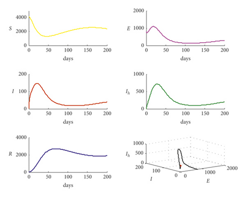
According to Figure 1, system (1) is settled at the endemic point when the basic reproduction number is R₀ = 2.4771, which means that the disease is out of control. However, for the data used in Table 1 with different values of parameter m, that m = 0,100,200,300, respectively, the trajectories of system (1) are drawn in Figure 2.

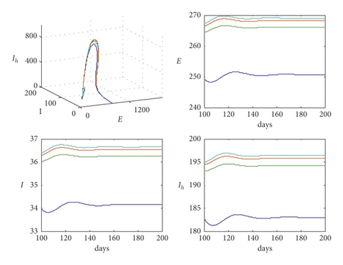
It is clear from Figure 2 that with the increase in the value of m, the trajectory still settled at endemic but the populations of exposed, infected, and hospitalized infected increased too.

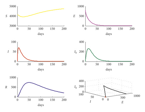
Now, for the data given in Table 2 with c = 0.9, it is observed that the basic reproduction number decreases to R₀ = 0.6193 and the trajectory of system (1) is shown in Figure 3. It is clear from Figure 3 that when R₀ < 1, system (1) approaches asymptotically to disease-free equilibrium point and that confirms the theoretical results in previous sections.

On the other hand, increasing the parameter b₁ from b₁ = 0.001 to b₁ = 0.01 with data used in Figure 3 makes the trajectory of system (7) return back to settle at the endemic equilibrium point as shown in Figure 4.

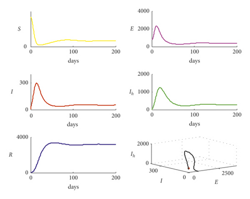
Clearly, from Figure 4, the bifurcation occurs in system (1) and the trajectory of system (1) transfers from disease-free point to endemic point as the bifurcation parameter b₁ increases, passing through the value and then becomes b₁ = 0.01. It is noted that the basic reproduction number increases from the value R₀ = 0.6193 to the value R₀ = 6.192717 passing the bifurcation value R₀ = 1. Now, for the data given in Table 2 with reducing the value of q from the value q = 0.5 to the value q = 0.2, the basic reproduction number decreases from the value R₀ = 2.4771 to the value R₀ = 0.9908, and the trajectory of system (1) is shown in Figure 5.

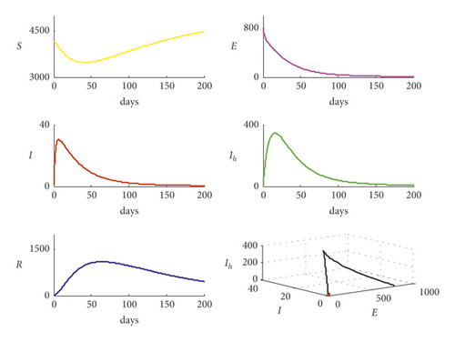
Again, Figure 5 ensures the obtained results regarding the stability analysis of the disease-free equilibrium point. Finally, other parameters are also varying to study their effects on the dynamical behavior of system (1), and it is observed that quantitative effects exist rather than qualitative one so that the population size of the different compartments in the system changes slightly.

8. Discussion and Conclusion

In this paper, an epidemic model to describe the spread of COVID-19 is proposed using the first-order ordinary differential equations. The model takes into account the impact of the curfew and media coverage on the control of the spreading of disease. It is observed that model (1) has two equilibrium points: the disease-free point that is stable, which means the disease is under control from a biological point of view, when the basic reproduction number satisfies R₀ < 1 and unstable for R₀ > 1, and the endemic equilibrium point that is stable, which means the disease out of control from a biological point of view, whenever the disease-free becomes unstable. All the properties of the solution of the model are studied. The local bifurcation near the disease-free point is investigated too. An application of the proposed model on the sample of Iraqi population of size 5000 has been done using baseline values of the parameters of system (1) as suggested by World Health Organization reports and adopted by many researchers, and the following observations are obtained.

The model has only one type of attractor, approaches either to disease-free equilibrium point or to the endemic equilibrium point, which means either stop the outbreak of COVID-19 or spread the COVID-19, depending on R₀ < 1 and R₀ > 1, respectively. The model is solved numerically using the Runge–Kutta fourth-order method with the help of Matlab. The model is applied to a sample of the Iraqi population using the parameter value ranges as suggested by the World Health Organization reports and adopted by many references as stated in Table 2. It is observed that increasing the probability of an individual’s response to the curfew leads to reducing the basic reproduction number below one and then controlling the spread of COVID-19, and hence system (1) approaches asymptotically to the disease-free point. However, increasing the direct contact rate between S and I in the absence of media alerts or decreasing the social distance between the population individuals leads to an increase in the basic reproduction number above one, and then an increase in the outbreak of the disease occurred. Hence, the trajectory of system (1) approaches the endemic point. Although increasing the response rate of the individuals to the media alerts (that means decreasing m) cannot prevent the disease from spreading completely, it leads to reduce it up to a minimum rate. A similar result is observed by increasing the parameter b₂, which increases the term (b₂I/m + I) that reduces the value of the transmission rate when infectious individuals appear and are reported. Finally, decreasing the fraction of the exposed individuals moving to the infected compartment, which leads to increasing the number of individuals moving to hospitalized infected populations, can prevent the disease from spreading and the system approaches a disease-free equilibrium point.

Conflicts of Interest

The authors declare that there are no conflicts of interest.

Open Research

Data Availability

The data used to support the findings of this study are included within the article.

References

1 WHO, Coronavirus Disease 2019 (COVID-19), 2019, WHO, Geneva, Switzerland, https://www.who.int/data#reports.
Google Scholar
2 Chowell G., Fenimore P. W., Castillo-Garsow M. A., and Castillo-Chavez C., SARS outbreaks in Ontario, Hong Kong and Singapore: the role of diagnosis and isolation as a control mechanism, Journal of Theoretical Biology. (2003) 224, no. 1, 1–8, https://doi.org/10.1016/S0022-5193(03)00228-5, 2-s2.0-0042168643.
10.1016/S0022-5193(03)00228-5
CAS PubMed Web of Science® Google Scholar
3 Carcione J. M., Santos J. E., Bagaini C., and Ba J., A simulation of a COVID-19 epidemic based on a deterministic SEIR model, Frontiers in Public Health. (2020) 8, https://doi.org/10.3389/fpubh.2020.00230.
10.3389/fpubh.2020.00230
PubMed Web of Science® Google Scholar
4 Eikenberry S. E., Mancuso M., Iboi E., Phan T., Eikenberry K., Kuang Y., Kostelich E., and Gumel A. B., To mask or not to mask: modeling the potential for face mask use by the general public to curtail the COVID-19 pandemic, Infectious Disease Modelling. (2020) 5, 293–308, https://doi.org/10.1016/j.idm.2020.04.001.
10.1016/j.idm.2020.04.001
PubMed Google Scholar
5 Maji C., Impact of media-induced fear on the control of COVID-19 outbreak: a mathematical study, International Journal of Differential Equations. (2021) 2021, 11, 2129490, https://doi.org/10.1155/2021/2129490.
10.1155/2021/2129490
Web of Science® Google Scholar
6 Asamoah J. K., Bornaa C. S., Seidu B., and Jin Z., Mathematical analysis of the effects of controls on transmission dynamics of COVID-19, Alexandria Engineering Journal. (2020) 59, no. 6, 5069–5078, https://doi.org/10.1016/j.aej.2020.09.033.
10.1016/j.aej.2020.09.033
Web of Science® Google Scholar
7 Peter O. J., Qureshi S., Yusuf A., Al-Shomrani M., and Idowu A. A., A new mathematical model of COVID-19 using real data from Pakistan, Results in Physics. (2021) 24, 104098, https://doi.org/10.1016/j.rinp.2021.104098.
10.1016/j.rinp.2021.104098
PubMed Web of Science® Google Scholar
8 Das P., Upadhyay R. K., Misra A. K., Rihan F. A., Das P., and Ghosh D., Mathematical Model of COVID-19 with Comorbidity and Controlling Using Non-pharmaceutical Interventions and Vaccination, Nonlinear Dynamics. (2021) 106, no. 2, 1213–1227, https://doi.org/10.1007/s11071-021-06517-w.
10.1007/s11071-021-06517-w
PubMed Web of Science® Google Scholar
9 Musa S. S., Baba I. A., Yusuf A., Sulaiman T. A., Aliyu A. I., Zhao S., and He D., Transmission dynamics of SARS-CoV-2: a modeling analysis with high-and-moderate risk populations, Results in Physics. (2021) 26, 104290, https://doi.org/10.1016/j.rinp.2021.104290.
10.1016/j.rinp.2021.104290
PubMed Web of Science® Google Scholar
10 Paul A., Reja S., Kundu S., and Bhattacharya S., COVID-19 pandemic models revisited with a new proposal: plenty of epidemiological models outcast the simple population dynamics solution, Chaos, Solitons & Fractals. (2021) 144, 110697, https://doi.org/10.1016/j.chaos.2021.110697.
10.1016/j.chaos.2021.110697
PubMed Web of Science® Google Scholar
11 Asamoah J. K. K., Owusu M., Jin Z., Oduro F. T., Abidemi A., and Gyasi E. O., Global stability and cost-effectiveness analysis of COVID-19 considering the impact of the environment: using data from Ghana, Chaos, Solitons and Fractals. (2020) 140, 110103, https://doi.org/10.1016/j.chaos.2020.110103.
10.1016/j.chaos.2020.110103
PubMed Web of Science® Google Scholar
12 Asamoah J. K. K., Jin Z., Seidu B., Sun G.-Q., Oduro F. T., and Alzahrani F., A mathematical model and sensitivity assessment of COVID-19 Outbreak for Ghana and Egypt, SSRN. (2021) 3612877, https://doi.org/10.2139/ssrn.3612877.
10.2139/ssrn.3612877
Google Scholar
13 Tang B., Bragazzi N. L., Li Q., Tang S., Xiao Y., and Wu J., An updated estimation of the risk of transmission of the novel coronavirus (2019-nCov), Infectious Disease Modelling. (2020) 5, 248–255, https://doi.org/10.1016/j.idm.2020.02.001.
10.1016/j.idm.2020.02.001
PubMed Google Scholar
14 Zhou F., Yu T., Du R., Fan G., Liu Y., Liu Z., Xiang J., Wang Y., Song B., Gu X., Guan L., Wei Y., Li H., Wu X., Xu J., Tu S., Zhang Y., Chen H., and Cao B., Clinical course and risk factors for mortality of adult inpatients with COVID-19 in Wuhan, China: a retrospective cohort study, The Lancet. (2020) 395, no. 10229, 1054–1062, https://doi.org/10.1016/s0140-6736(20)30566-3.
10.1016/S0140-6736(20)30566-3
CAS PubMed Web of Science® Google Scholar
15 Liu Y. and Cui J.-A., The impact of media coverage on the dynamics of infectious disease, International Journal of Biomathematics. (2008) 1, no. 1, 65–74, https://doi.org/10.1142/s1793524508000023, 2-s2.0-84863116523.
10.1142/S1793524508000023
Web of Science® Google Scholar
16 Diekmann O., Heesterbeek J. A. P., and Metz J. A. J., On the definition and the computation of the basic reproduction ratio R₀ in models for infectious diseases in heterogeneous populations, Journal of Mathematical Biology. (1990) 28, 365–382, https://doi.org/10.1007/bf00178324, 2-s2.0-0025159677.
10.1007/BF00178324
CAS PubMed Web of Science® Google Scholar
17 Driessche P. V. D. and Watmough J., Reproduction numbers and sub-threshold endemic equilibria for compartmental models of disease transmission, Mathematical Biosciences. (2002) 180, no. 1-2, 29–48, https://doi.org/10.1016/s0025-5564(02)00108-6, 2-s2.0-0036845274.
10.1016/S0025-5564(02)00108-6
PubMed Web of Science® Google Scholar

Citing Literature

All articles

The Impact of Media Coverage and Curfew on the Outbreak of Coronavirus Disease 2019 Model: Stability and Bifurcation

Abstract

1. Introduction

2. Formulation of the Model

3. Existence of the Equilibrium Points and Basic Reproduction Number

4. Local Stability Analysis

5. Global Stability

6. The Local Bifurcation Analysis

7. Numerical Simulation

8. Discussion and Conclusion

Conflicts of Interest

Open Research

Data Availability

References

Citing Literature

Figures

References

Information

About Wiley Online Library

Help & Support

Opportunities

Connect with Wiley

The Impact of Media Coverage and Curfew on the Outbreak of Coronavirus Disease 2019 Model: Stability and Bifurcation

Abstract

1. Introduction

2. Formulation of the Model

3. Existence of the Equilibrium Points and Basic Reproduction Number

4. Local Stability Analysis

5. Global Stability

6. The Local Bifurcation Analysis

7. Numerical Simulation

8. Discussion and Conclusion

Conflicts of Interest

Open Research

Data Availability

References

Citing Literature

Figures

References

Related

Information