1. Introduction

Point cloud is a collection of points. It contains rich information, which can be three-dimensional coordinates X, Y, Z, color, intensity value, time, and so on. Point clouds are representative of geometric data structures. In this paper, we use deep learning network structures to perform feature extraction and recognition for each point cloud object in a realistic scene.

Compared with other methods, most of the objects in point cloud scene model in this paper have no repeated occlusion. Euclidean distance clustering segmentation methods can be used to segment objects in complex scenes. The samples n points require as much original feature information as possible, so the Monte Carlo method is used. Using the deep learning network structure proposed in this paper to directly recognition point cloud objects can greatly reduce the amount of data calculation (compared to mainstream methods such as converting point clouds to regular depth maps, multiviews, or voxel grids). Point clouds do not introduce quantization artifacts, which can better maintain the natural invariance of data. The experimental results show that the network structure in this paper can accurately identify and classify point cloud objects in realistic scenes and maintain a certain accuracy when the number of point clouds is small, which is very robust.

The deep learning network structure proposed in this paper to identify point cloud objects is a systematic method. The three-dimensional coordinates of n points of a point cloud object are input to a deep learning network, and local features or global features are extracted and added to other dimensions to identify and classify point cloud objects in a realistic scene. Before the point cloud object is input into the deep learning network structure, each point of the input is preprocessed identically and independently, and each point of each point cloud object includes information of only three coordinates.

The realistic scene in this article is shown in Figure 1. The point cloud diagram of the realistic scene in this paper is shown in Figure 2. Figure 3 is a single-point cloud object after segmenting the realistic scene in this paper using Euclidean distance clustering segmentation. A single-point cloud object segmented using Euclidean distance clustering is input to the deep learning network trained in advance in this paper, and the global features of a single point cloud object are extracted through the max-pooling layer in the network structure. Then, the multilayer perceptron connected through the fully connected layer performs classification and recognition of the point cloud object on such learned features.

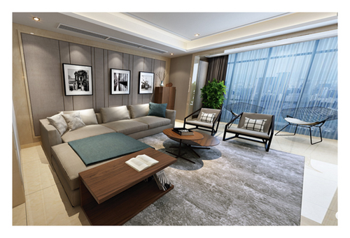
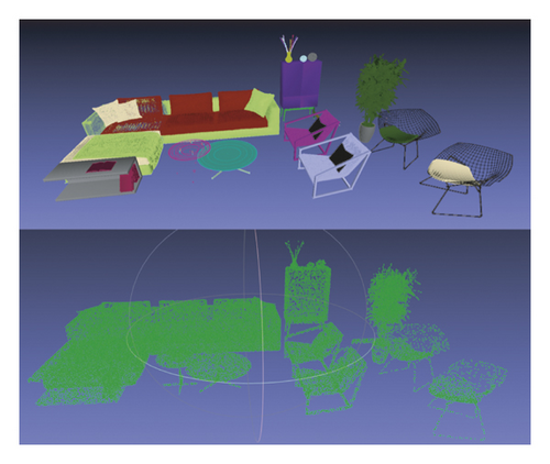
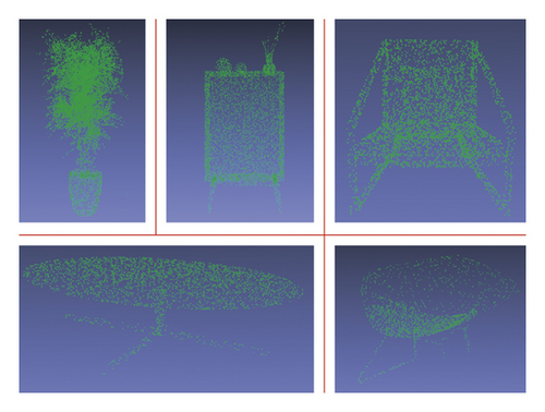
The input data format is easy to use rigid or affine transformation, so the experiment results can be further improved. For the realistic scene and network structure adopted in this paper, this paper provides both theoretical basis and numerical evaluation.

The rest of this article is organized as follows: Section 2 reviews various methods proposed in the literature for different forms of 3D data; Section 3 describes two main problems addressed in paper; Section 4 proposes a solution to the first problem in Section 3; Section 5 proposes a solution to the second problem in Section 3; Section 6 mainly analyzes the experimental results and the robustness of the proposed network method; and Section 7 illustrates the deficiencies in the experiment and suggests work to be done next.

2. Related Work

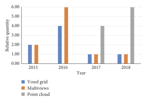
There are three main methods for 3D object recognition, which are based on 3D voxel grid, collections of images, and point cloud data. The point cloud learning-based approach is currently getting more accurate as shown in Figure 4, and the number is growing dramatically as shown in Figure 5. In addition to these methods, there are some other methods such as spectral convolutional neural network (CNN), feature-based deep neural network (DNN), etc.

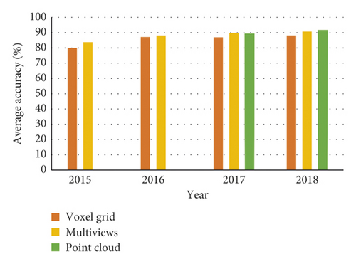
Methods based on collections of images data are as follows. The main research is to use the geometric method to transform a three-dimensional object into several multiview geometric two-dimensional images and retain as much feature information as possible. In addition, in recent years, many deep learning algorithms are mostly based on two-dimensional images, and many excellent research results have appeared in two-dimensional images. Qi et al. and Su et al. [1, 2] attempt to convert a 3D point cloud object into multiple different 2D images and then design a new convolutional neural network algorithm structure to integrate the view information of multiple 2D images into a compact shape descriptor. Yi et al. [3] uses multiple views to represent local information on the graph by parameterizing kernels in the spectral domain spanned by the characteristic roots of the graph. Experiments have shown that all benchmark datasets in each task achieve state-of-the-art performance.

Methods based on the 3D voxel grid data are given as follows: this method works by meshing or voxelizing various 3D data and then designing the corresponding 3D convolutional neural network for feature extraction and recognition. References [1, 4–7] is a series of convolutional neural network algorithms whose input data is a voxel grid, but these algorithms all consume a lot of computational costs because of the sparseness of the data and the features of convolution in 3D. The requirements for resolution are high. FPNN [8] and Vote3D [9] have proposed different solutions to the problem of sparsity of voxel grid data. However, these two schemes are not very ideal, and the experimental results are not very satisfactory, so it is still a very big challenge to process point cloud data with a very large amount of data.

Methods based on the point clouds. This method mainly includes two types. One is to convert the point cloud data into a multiview, polygon network, or voxel grid and then use deep learning networks for feature extraction and recognition (as described above). The other part is to directly process the point cloud data. The recognition accuracy is high and there is development in speed in the last three years. Qi et al. [10] are the first to directly process the point cloud data, avoiding the unnecessary huge problem of the data and well respecting the replacement and deformation of the input points. Based on this, they proposed a new neural network structure PointNet [10] and PointNet++ [11] to directly process point cloud data. Based on the principle of kdtree, Klokov and V. Lempitsky [12] propose a network algorithm Kdnetwork that is different from the current mainstream convolution structure. It uses rasterization on a uniform two-dimensional or three-dimensional grid to avoid bad scaling behavior for 3D models and point clouds. Identifying tasks is explained as follows. Zaheer et al. [13] mainly propose a series of permutation invariant functions that can be run on a set. This series of permutation invariant functions can be used in various positions. Among the various algorithms that process point cloud data, the best and the most accurate are PointCNN [14] proposed by researchers at Shandong University based on convolution operators in convolutional neural networks. PointCNN uses χ transform to weight the input features associated with points, which works very well in classification and segmentation scenes.

For spectral CNN [15–17], at present, this series of methods is only applicable to convolutional neural networks such as organic matter. Feature-based DNNs (deep neural networks) [18,19] usually convert a series of 3D data features into appropriate features and then use a fully connected layer to classify and recognize the point cloud data. In summary, CNN can extract high-level semantic information from the original data through a series of operations such as convolution and pooling and finally generate a valid feature. It aims to improve the classification accuracy of large-scale multicategory complex 3D models. Firstly, the three-dimensional polygon mesh model is discretized into three-dimensional point cloud data, and then the deep feature of the model is extracted by convolution and pooling of the deep point cloud convolutional neural network, and the model is classified and identified by using multilayer perceptron.

On the Generation of Point Cloud Data Sets: Step One in the Knowledge Discovery Process [20], Andreas Holzinger et al. describe the case for natural point clouds and then provide some fundamentals of medical images, particularly dermoscopy, confocal laser scanning microscopy, and total-body photography; they describe the use of graph theoretic concepts for image analysis, give some medical background on skin cancer, and concentrate on the challenges when dealing with lesion images and the discussion of related algorithms. The point cloud data is extracted from different weakly structured sources and topologically analyzed to produce feasible results. The quality of these results depends not only on the quality of the algorithm itself, but also to a large extent on the quality of the input maps they receive, so point clouds are a necessary preprocessing step and affect the quality of the experimental results.

3. Problem Statement

In order to complete the recognition of point cloud objects in realistic scenes, two key problems need to be solved. The first key question: how to separate multiple point cloud objects in a realistic scene. Since the object input to the deep learning network is a complete point cloud object, and each point cloud object in the realistic scene is clustered together, an algorithm needs to be designed to segment multiple point cloud objects in the scene into a single. It is mainly based on the information that each point cloud object has different textures and colors to segment and save to each separate file and then input each individual point cloud object to the trained deep learning network for classification and recognition.

The second key issue is to design and propose a new deep learning network structure for point cloud data to process it directly. After solving the first critical problem mentioned above, we will obtain a single point cloud object for preprocessing, and then input each point of the point cloud object to the trained deep learning network for classification and recognition. Point cloud is a collection of x, y, and z coordinates, as well as color, normal vectors, and other feature channel feature information. For the convenience of processing and clarity, this article only uses the three coordinates (x, y, z) of each point as the input of the deep learning network.

4. Euclidean Distance Clustering Segmentation and Data Preprocessing

Euclidean distance clustering segmentation and data preprocessing are divided into two parts. First, the working principle of Euclidean distance clustering segmentation algorithm is introduced (Section 4.1). The method has a better effect in a realistic scene with less overlap. Second, all point cloud objects are processed identically and independently. These processing methods mainly include Monte Carlo sampling, zero mean, and normalization (Section 4.2).

4.2. Data Processing

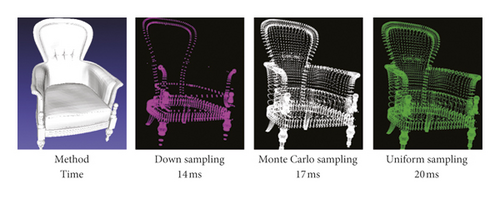
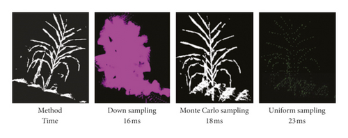
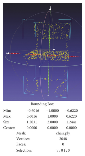
After performing Euclidean distance clustering and segmentation on a realistic scene, there will be many different point cloud objects, and these point cloud objects are composed of different numbers of points. Because of the premise of a network that recognizes point cloud objects: each point cloud object has the same number of points, so you need to use the sampling method to sample each point cloud object into n points. The n points after sampling are zero-mean and normalized. Each object is processed into a uniform format and entered into a network algorithm. The choice of sampling method is crucial. The sampling methods mainly considered in this paper are Monte Carlo sampling, downsampling, and uniform sampling. These three methods are used to sample the same object into 1024 points. The results after sampling and the time spent sampling are shown in Figure 6. The figure clearly shows that the Monte Carlo sampling method and uniform sampling can better show the contours and shapes of point cloud objects. However, when there are a large number of point clouds and each point contains more dimensional information, the unified sampling method requires greater computational cost and time cost. Taking the above two points into consideration, the method of sampling point cloud objects in this paper uses the Monte Carlo sampling method.

The main content of the Monte Carlo sampling method is to use Monte Carlo ideas to maximize the approximation of a series of data. That is, the point cloud is sampled, and the sampled points must retain the information of the original point cloud to the greatest extent. The larger the number of sampling points, the more accurate the approximation result is and the more it matches the distribution of the points in the original point cloud. For the theory of Monte Carlo sampling in this paper, the proof and algorithm are implemented as follows.

For any given function h(x), it can also be said that any point cloud object needs to be sampled. We need to approximate the value of this function. The first integral to be calculated is

$$ ()

Since there is no way to solve this equation using mathematical derivation, it should be noted that for all x values on the interval, the product of the function f(x) and the probability density function p can be used instead of the function h(x). So the entire integral can be written as

$$ ()

where p’s expectations are E_p, probability distribution p for random variable x. So the mean of f(x) on the p distribution is equivalent to the original integral. At this time, a series of sampling sample points x⁽¹⁾, x⁽²⁾, …, x⁽ⁿ⁾ is used to approximate s. From these points, the empirical average is calculated as

$$ ()

and the collected sample points are used to approximate the average mean:

$$ ()

The following theories can clearly prove the legitimacy of this approximation. It is clear that the estimate of $$ is correct and without bias,

$$ ()

that is,

$$ ()

and the above formula only needs to satisfy that the variance of each individual variable Var[f(x⁽ⁱ⁾)] is bounded. Further, when we consider that the n increases, as long as the variance of $$ satisfies Var[f(x⁽ⁱ⁾)] < ∞, the variance $$ will decrease and must converge to 0:

$$ ()

For a random variable X, if there is a defined function F,

$$ ()

Regarding the continuous random X as the cumulative distribution function of F(x), if there is a function f(x) defined on the real axis and is nonnegative, for any real number x, the following formula is established:

$$ ()

Therefore, the cumulative distribution function of the probability distribution can usually be obtained by integrating the probability density function. If you need to get n samples, repeat the following steps n times. (1) The computer can randomly sample a value from the point cloud data, expressed in μ. (2) Calculate the value x of F⁻¹(u), where x is a sample point derived from f(x).

Zero mean and normalization (which can get better experimental performance) is a necessary step before training the neural network. Generally, the sample data obtained has multiple dimensions. That is, one sample is represented by multiple features. The original data is directly used in training, and their influence on train results is different. By zero mean and normalization, different features can have the same scale. When the gradient descent method is used to update the parameters, different types of features have the same level of influence on parameters. Zero mean and regularization can accelerate the convergence of weight parameters during training. Zero mean is a set of data, each of which is subtracted from the average of this set. Assume that a series of samples of the data is x_i. The zero mean of the data is as follows:

$$ ()

In order to bring all data under a unified standard, we use min-max scaling to normalize all data to [−1,1]:

$$ ()

where the normalized data is X_norm, the original data is X, the maximum value of the raw data is X_max, and the minimum value of the raw data is X_min. The results after zero-mean and normalization are shown in Figure 7.

5. Deep Learning on Point Sets

Deep learning on point sets are divided into two parts. First, Section 5.1 introduces two main problems, solutions and proofs, in the process of deep learning processing point sets. Second, Section 5.2 introduces the improved network structure for identifying objects.

5.1. Problems of Point Sets in ℝⁿ

All data in the point cloud are a collection of points from European space. The point set of these Euclidean spaces will encounter two key problems: the disorder of the point cloud and the invariance of rotation and translation during the processing of the algorithm. This article gives corresponding solutions to these two problems.

5.1.1. Unordered

Affected by the acquisition equipment and the coordinate system, the same object is scanned using different equipment or positions, and the order of the three-dimensional points varies greatly. The point cloud data is very different from the pixel arrangement in the two-dimensional image or the voxel arrangement in the voxel grid. Point cloud is a set of points without a fixed order. When using a deep learning network to perform different tasks on a point cloud, no matter in what order it is input to the network, the same results must be output. In RGB-D or grayscale images, the relative position of each pixel is fixed, and there is no problem of disorder. However, for point cloud data, there are N! types for entering points into the network using a different order. Therefore, the input point cloud data needs to be processed accordingly.

There are three solutions to the disorder of point cloud data. (1) Input the point cloud data in a certain order. (2) With the help of recurrent neural network, increase the training data by adding various permutations. (3) Aggregate the information of each point with the help of some common symmetric functions. Suppose there is such a sorting strategy, which will define a mapping graph in one-dimensional space and high-dimensional space. It is easy to see that when the size is reduced, both the sequence stability and the point perturbation are required to maintain the proximity of the space, which is an impossible task in practical situations. Therefore, strategy one cannot solve the disorder problem of point cloud data. With the idea of recurrent neural networks and hope to train recurrent neural networks by randomly permuting sequences, the author has already stated that order is very important in OrderMatters, and it cannot be ignored, although recurrent neural networks have a good effect on relatively small sequences, but scaling to thousands of input elements is difficult. For using the symmetric function to solve the disorder problem of point cloud data, this strategy has been verified in the PointNet classification network [10] and has a good effect. Therefore, the solution adopted in this article is to solve the disorder problem of point cloud data by using a symmetric function. The symmetric function used is the following formula:

$$ ()

where f2^ℝ⟶ℝ, the feature extraction layer is represented by h, the symmetric method using the max-pooling layer is represented by g, higher-dimensional feature extraction is represented by γ. The symmetric function used in this paper has simple modules: a multilayer perceptron to approximate h, a maximum pooling function, and a variable function to approximate f. By collecting h, the deep learning network can learn various feature attributes of different objects through f. In other words, the feature of the last higher dimension is to choose the largest feature value in each dimension to solve the disorder problem of the point cloud data, that is, g.

Theorem 1. Suppose f is a continuous set function about Hausdorff distance d_H, ∀ε > 0, ∃ a continuous function h and asymmetric function g(x_i, …, x_n = γ∘Max), such that for any W ϵ Q,

$$ ()

Formally, letQ = {W : W⊆[0,1]^m and |W| = n}, f : Q⟶ℝ is a continuous set function on Q about Hausdorff distance d_H, ∀ε > 0, ∃δ > 0, for any W, W^′ϵQ, if d_H(W, W^′) < δ, then |f(W) − f(W^′)| < ε.

5.1.2. Rotation and Translation Invariance

Point cloud is a geometric object. If the point cloud undergoes certain geometric transformations (such as rotation and translation operations), the semantic label of point cloud classification and segmentation must be constant. Therefore, we expect our learning of the point set to be invariant to these transformations.

For the invariance of rotation and translation of point cloud data, the natural solution is to align all input sets with the canonical space before feature extraction. Jaderberg et al. [21] introduces the idea of spatial transformer to align 2D images by sampling and interpolation, through a specially customized layer implemented on the GPU. This paper uses the adjustment network proposed by Qi et al. [10] to solve this problem, and the effectiveness of this solution has been proved in the paper. The affine transformation matrix can be predicted by adjusting the network, and the predicted affine transformation matrix can be used for the input of the point cloud. However, it should be noted that the transformation matrix of the feature space has higher-dimensional features, which greatly increases the difficulty of optimization, so it is necessary to reduce the difficulty of optimization by adding a regular loss:

$$ ()

where the feature alignment matrix of the adjustment network is A. The orthogonal transformation of the above formula can largely preserve the original information.

After adding regular terms, not only can you get a more stable solution, but also reduce the parameters to a large extent.

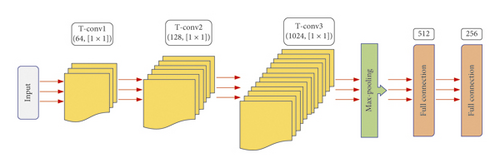
The schematic diagram of adjusting the network structure is shown in Figure 8. The adjustment network is a subnetwork used to predict the transformation matrix in the feature space. It learns the transformation matrix that is consistent with the feature space dimension by learning from the input data, which multiplies the learned transformation matrix with the original data. The transformation operation in the data feature space causes each point of the subsequent input to be associated with each point in the input. Through such processing, the feature inclusion in the input point cloud data is hierarchically abstracted. The adjustment network consists of three convolutional layers, one max-pooling layer, and two fully connected layers. Convolution layer 1 has 64 feature maps, convolution kernel is [1 × 1]; convolution layer 2 has 128 feature maps, convolution kernel is [1 × 1]; convolution kernel 3 has 1024 feature maps, and convolution kernel is [1 × 1] The full connection layer is 512 and 256 nodes, respectively.

5.2. Network Architecture

Because PointNet’s [10] classification and segmentation network has achieved good results and its ability to extract features is very strong, it motivates our recognition requirements for point cloud objects in realistic scenes. This article draws on the classification network of PointNet. The adjustment of the structure of this network in this paper makes the network further enhance the feature extraction ability. The experimental results show that the proposed deep learning network structure can improve the accuracy of point cloud object classification and recognition, while also greatly improving the accuracy on the training and testing sets. The network structure is shown in Figure 9. The input data is the 3D coordinates of a series of point sets for each point cloud object. The max-pooling layer solves the problem of disorder of point cloud data and adjusts the network to solve the problem of rotation and translation invariance of point cloud objects. The structure of feature extraction for point cloud objects is accomplished through a combination of multilayer perceptrons and adjustment networks. The max-pooling layer can also obtain the global characteristics of each object. Through this process, the point cloud object recognition in the realistic scene is completed.

The main part of feature extraction in Figure 9 includes three adjustment networks, a maximum pooling layer, and three multilayer perceptrons, which are input through the three-dimensional coordinates of n points. The features are extracted, and the extracted features are mapped to a column vector through the maximum pooling layer to complete the feature extraction of the point cloud data. In order to complete the task of identifying and classifying point cloud data, it is necessary to perform probabilistic calculations on the features extracted by the deep network architecture. Therefore, it is necessary to connect the fully connected layer after the maximum pooling layer to map the learned feature representation to the sample tag space. In the figure, the first fully connected layer contains 512 neurons, the second fully connected layer contains 256 neurons, and the number of the third fully connected layer neurons is the number of categories for the classification task. The dropout layer is set to zero for each neuron node with a probability of 70%. At this time, the effect is also the best. This can alleviate the complex collaborative adaptation between neurons, reduce neuron dependencies, and avoid network training. Overfitting occurs during the process. In addition, the generalization ability of the model can be improved and the complexity of the model can be reduced.

Softmax has a wide range of applications in deep learning. Especially when solving multiclassification tasks, the final output unit of the classifier needs to use the Softmax function for numerical processing to convert the output values of multiple classifications into corresponding probabilities. The definition of the Softmax function is

$$ ()

where b_i is the output of the superior output unit of the classifier; i is the index value of the category; C is total numbel of categories; S_i is the ratio of the index of the output element of the previous output unit of the classifier to the sum of the index of all elements.

The loss function used in this article is as follows:

$$ ()

where y_i is the true classification result; S_i is output of Softmax function. After the calculation of the cross-entropy loss is completed through the above formula, the weight of the network is adjusted using the back-propagation algorithm.

6. Experiment

Experiments are divided into two parts. First, Section 6.1 provides detailed training process. Second, Section 6.2 analyzes the experimental results and tests the robustness of the network.

6.1. Training Process

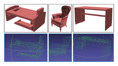
In this paper, in order to train the deep learning network structure, we choose the ModelNet [22] data set established by Stanford University as the training set and test set for network learning. ModelNet data has 40 different kinds of 3D models and each has a corresponding number, and there are 12, 311 3D objects in total. We then divide these models into 4 files with, 64 group per file and 32 models per group. The remaining 2048 model files are used as test sets. They were written in a file in the same way. These files are entered into the network and trained. Figure 10 shows some of the model files in ModelNet40 and the point cloud files that have been processed for training. During the training of deep learning network algorithms, point clouds are randomly rotated along the upper axis and point clouds are dynamically added by adding Gaussian noise.

In addition, you need to set some basic parameters of the network and explain the evaluation indicators of the results after the training is completed. Optimize the network by using a momentum-based stochastic gradient descent method. The momentum factor is set to 0.9, the weight attenuation is 0.0005, the initial learning rate is 0.001, and the dropout rate is 0.7. The network parameters are initialized using random initialization. After the training is completed, the trained parameters of the network are obtained, and then the trained network is used to test the data collected by the machine vision platform through the recognition and classification task. The performance index of the test uses the accuracy rate and is defined as follows:

$$ ()

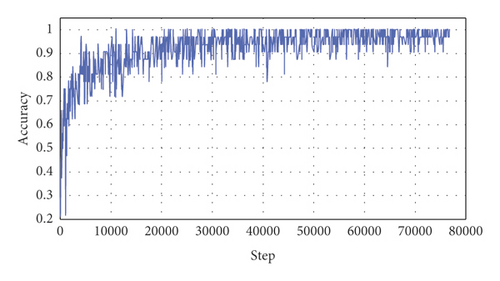
The server hardware configuration for deep learning network training is as follows: Ubuntu 18.04 system, 8-core 16-thread Inter Core i7 − 5960 X processor, 2 NVIDIA M 4000 graphics cards, 16 GROM, TensorFlow 1.7.0 [23]. The training process record of the entire deep learning network algorithm is shown in Figure 11 below.

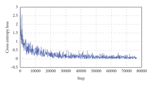
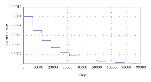
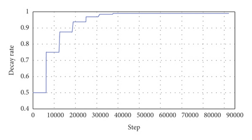
Due to the particularity of deep learning networks, setting different parameters for the same deep learning network will have different results. In order to reproduce the experimental results, record the parameter settings of the deep learning network before training in this paper in Table 1.

Table 1. The initial and end values of some parameters during the training process.

	Initial value	End value
Accuracy	0	0.988
Cross-entropy loss	1.9408	0.024
Learning rate	0.001	0.0000133
Decay rate	0.5	0.982

6.2. Results and Analysis

After the deep learning network training is completed, the preset test set is used to test the recognition accuracy. There are three main indicators: average loss, average accuracy, and average classification accuracy. The test results are shown in Table 2.

Table 2. Results on the test set.

Average loss	0.5014
Average accuracy	0.897
Average classification accuracy	0.873

The experimental results in this paper are compared with the better method of idle money. The comparison results are shown in Table 3.

Table 3. Comparisons of classification accuracy (%) on ModelNet40.

Method	Input	ModelNet40 (%)
FPNN [8]	Volume	68.20
3DShapeNets [22]	Volume	77.30
VoxNet [4]	Volume	83.00
Subvolume [1]	Volume	86.00
PointNet(vanilla) [10]	Point cloud	87.20
PointNet [10]	Point cloud	89.20
This paper	Point cloud	89.70

The task of this paper is to identify point cloud objects in realistic scenes. Table 4 below is an analysis of the accuracy of recognition objects that may appear in realistic scenes.

Table 4. Results on the test set.

Bed	Guitar	Cup	Bottle	Bowl	Curtain
0.99	0.94	0.70	0.70	0.99	0.90
Bookshelf	Person	Door	Keyboard	Plant	Piano
0.91	0.95	0.85	0.85	0.80	0.87
Chair	Laptop	Lamp	Sofa	Desk	Wardrobe
0.98	0.99	0.95	0.97	0.99	0.55

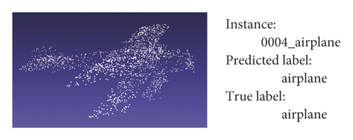
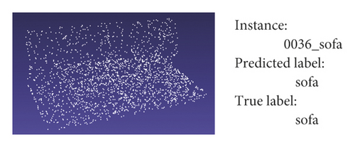
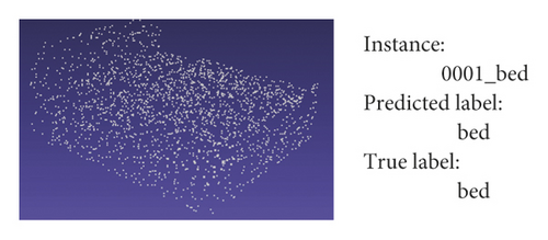
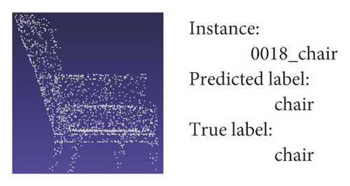
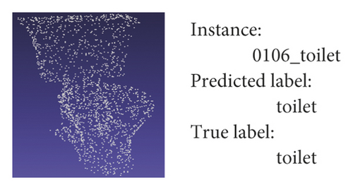
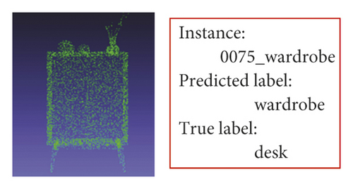
Table 4 shows the method used in this paper to identify some point cloud objects in the realistic scene and the accuracy rate of recognition. It has a high accuracy rate for some objects with obvious features. In short, the method in this paper can accurately identify objects in realistic scenes. Figure 12 shows an example of point cloud object recognition in the real scene by the algorithm in this paper. Recognize the objects in the realistic scene, the main information and results of the recognition are shown in Figure 13.

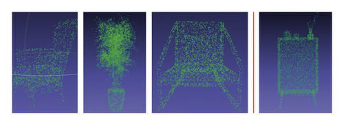
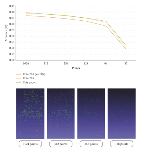
In order to test the robustness of the network algorithm in this paper, we test the accuracy of the point cloud object recognition by gradually reducing the number of each point cloud object. Ideally, as the number of point clouds decreases, the accuracy is maintained as much as possible. Through experiments, we find that with the reduction of the number of point clouds, the accuracy of point cloud object recognition gradually decreases, but the accuracy of recognition is maintained at a high level. Even with only 64 points of information, the accuracy rate remains above 60%. The robustness test of the deep learning network in this paper is shown in Figure 14.

7. Conclusion

This paper proposes a new approach to recognize point sets objects in realistic scenes by clustering and segmenting point cloud data in realistic scenes using on the Euclidean distance clustering segmentation algorithm. It effectively solves the problem of clustering and segmentation of multiple objects in complex scenes. Using a deep learning network that directly processes point cloud greatly reduces the amount of data calculation. Point cloud does not introduce quantization artifacts, which can better maintain the natural invariance of data. The experimental results show that the network structure in this paper can accurately identify and classify point cloud objects in realistic scenes and maintain a certain accuracy when the number of point clouds is small, which is very robust. For any point cloud object has global features and local features, the algorithm proposed in this paper mainly extracts global features and does not make use of local features. In the next work, we want to further change the network structure to extract local features and further improve the accuracy of point cloud object recognition in realistic scenes.

Conflicts of Interest

There are no conflicts of interest regarding the publication of this manuscript.