Wind farm siting relies on in situ measurements and statistical analysis of the wind distribution. The current statistical methods include distribution functions. The one that is known to provide the best fit to the nature of the wind is the Weibull distribution function. It is relatively straightforward to parameterize wind resources with the Weibull function if the distribution fits what the function represents but the estimation process gets complicated if the distribution of the wind is diverse in terms of speed and direction. In this study, data from a 101 m meteorological mast were used to test several estimation methods. The available data display seasonal variations, with low wind speeds in different seasons and effects of a moderately complex surrounding. The results show that the maximum likelihood method is much more successful than industry standard WAsP method when the diverse winds with high percentile of low wind speed occur.

1. Introduction

One of the first and most crucial steps for wind farm investment is to investigate the characteristics of the local wind resources. The aim is to select the optimum locations for the turbines, maximizing income and minimizing cost. The analysis most commonly relies on in situ measurements collected through conventional meteorological masts (met. masts) [1, 2]. Recently, remote sensing devices with vertical wind profiling capabilities have also been accepted by the market, but these devices have limitations, mostly related to the complexity of the terrain [3–6]. Therefore, the methodology of spatial modeling based on point measurements is practically the only acceptable methodology for the wind site assessment step. A conventional met. mast is usually erected on a location that is considered representative of the area of interest. Sometimes more than one met. mast may be necessary if the wind characteristics are particularly variable in an area. Cup anemometers, vanes, sonics, and atmospheric sensors are used as measurement devices. It is important that data collection has a high recovery rate in order to accurately capture the wind resources, and a rate of 90% is ideally preferable. The final aim is to use the collected data for creating sector wise and generalized wind statistics for the measurement location. The generalized wind statistics can be used to create regional wind climates, also known as wind atlases. Since the atlas represents the larger domain, one can statistically transfer the in situ measurements to desired wind turbine locations. After several iterations of the process, the best production numbers are calculated, which will maximize the income of the wind farm

For many years, wind data have been represented by the Rayleigh distribution function [7, 8]. Although they are similar and come from the same statistical methodology, for almost over three decades, the Weibull distribution function has been the choice of experts, mainly because it is considered to be more representative of the natural wind characteristics [9]. One of the first studies that used the Weibull function as the main statistical methodology was the European Wind Atlas [10], which leads to the industry standard Wind Atlas Methodology. The Weibull distribution function (equation (1)) can be presented as a cumulative (CDF) (equation (2)) or probability (PDF) (equation (3)) density distribution function where U is the wind speed, A is the scale of the wind speed (m/s), and k is the unitless shape parameter [11].

(1)

(2)

(3)

The common way of using the distribution function is to fit measured wind speed frequency data to the probability density function to get the relationship between the wind speed and the wind frequency with two-parameter Weibull distribution. Thereafter, one can define the observational climate of the location by only recording two characteristics, A and k.

Although the method looks straightforward, there are known problems. The most important one is diverse wind conditions, occurring with high frequency during the year, which add extra uncertainty to computational fitting parameters; this is the case in all used methods [12]. In this study, a dataset with high recovery rate from a semicomplex terrain at 101 m height was used to compare different estimation methods of the Weibull parameters. The aim was to perform a comparison between the most widely used methods for a representative height for common wind turbines.

In the next section, studies on distribution function for wind energy use and specifically Weibull distribution are discussed, followed by the experimental setup and presentation of available wind data used with five different estimation methods. Finally, the results are compared and discussed.

2. Experimental Setup and General Wind Characteristics

Izmir Institute of Technology (IZTECH) is located on the west coast of Turkey, around 40 km to the west of the city of Izmir at the village of Urla. The peninsula surrounding the area has more than 20% of the total installed wind power capacity of Turkey. In August 2017, a mast with 101 m height was erected in the university campus with several instruments mounted (Table 1) at N38.3332° E26.6326° geographic coordinates. The reasoning of the new met. mast is to make academic studies about wind speed distributions, atmospheric stability, and complex terrain short-term predictions. Therefore, the mast is equipped with also two 3D sonic anemometers and measurement devices in different heights.

Table 1. Available instrumentation on the IZTECH met. mast with recovery rate for the period between 21 December 2017 and 21 December 2018. The wind speed and the wind direction are measured with sonic 3D anemometer at 10 m and 52 m, while other heights are measured with conventional anemometers.

Parameter	Unit	Heights (m)
Wind speed	(m/s)	101, 76, 52, 30, 10
Wind direction	°	98, 74, 52, 28, 10
Temperature	(°C)	90, 35, 3
Relative humidity	(%)	90, 35, 3
Pressure	(Pa)	90, 2

Data collection started on the 1st of August 2017 and the campaign is ongoing. The best recovery rate, with over 99.9% for a full year’s data, is available between the 21st of December 2017 and the 21st of December 2018, totaling 52191 of 10-minute samples. The available data were filtered with two rules: (i) the standard deviation of the channels is bigger than zero and (ii) wind speeds below a calm threshold level for cup and vane of 0.3 m/s and 0.4 m/s, respectively, are ignored; meanwhile, the final recovery rate for the channels dropped down to 99%. The data can be considered to be of high quality in terms of availability. The air density was measured to be 1.19 kg/m³ on average and only changes ±0.01 kg/m³ throughout the day in monthly and yearly average but can sometimes reach 1.01 kg/m³ in the occasional 10-minute sample.

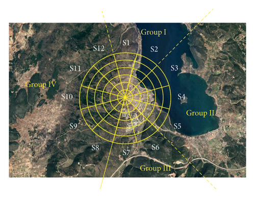
The location of the met. mast was chosen for research purposes (Figure 1), such that each wind sector has different combinations of terrain and roughness classifications. The main wind direction is the first sector, S1, where the northerly wind occurs more than 45% of the time. S1 is located 5 km away from coastline and has a flat terrain at 50 m a.s.l., covered with grass. S2 is only 1 km away from the coastline and is under the influence of the sudden roughness change. S3, S4, and S5 are occupied by a small village with narrow streets, where the tallest houses are approximately 6.5 m high. The village is built parallel to the coastline and the sea is nearly 1.25 km from the met. mast at its closest location. S6 and S7 are occupied by the IZTECH campus, with the buildings closest to the mast being 4 m high at maximum, while further away (> 12 m distance), there are taller university buildings but more sparsely located. A hill parallel to the coastline with an average height of 350 m a.s.l. covers the grounds of S8–S12. The vegetation of these sectors is characterized by low bushes (max. 30 cm) mixed with grassland. The only unique sector within this range is sector S9, where 5 units of 3 MW wind turbines are located more than 5 km away from the mast. Due to the long distance, it is assumed by the author that the met. mast is not under the influence of these turbines (Table 2).

Details are in the caption following the image — **Figure 1**
Open in figure viewer PowerPoint

The center being the met. mast location: the figure shows up to 3 km radius with 500 m circle steps size. Wind sectors are split into 12 wind direction sectors, 30° each, starting from first sector being centered at 0°. White numbers are the sector numb.

Table 2. Sector-wise wind frequency and topographical characteristics. The sectors are grouped based on similarities of roughness and obstacles.

Sector	Center	Fre. (%)	Group	Terrain	Roughness	Obstacles
1	0	45.65	I		Grassland	None
2	30	11.21	I		Grassland	Small cottages

3	60	1.95	II	Flat; 50 m a.s.l.	Urban area	Village with max 6.5 m tall houses
4	90	1.41
5	120	1.3

6	150	3.7	III			University with tall buildings
7	180	12.59	III			University with tall buildings

8	210	7.59	IV	Hilly; up to 350 m a.s.l. with gentle slope	Grassland	None
9	240	2.75				Distant wind farm
10	270	2.09				None
11	300	4.66
12	330	5.07

Vertical wind profiles were calculated with all the data and the yearly statistics show an almost logarithmic vertical wind speed profile except for the minor speed up at 30 m height (Figure 2(a)). The wind directional turn shows minor terrain effects above 50 m where the averaged wind direction becomes nearly stable (Figure 2(b)). All five wind speed channels were also analyzed for diurnal statistics, which demonstrate that the measurement location is characterized by an almost laminar flow at night and quite unstable conditions during daytime (Figure 3). Based on the yearly averaged wind speed values, the omnidirectional wind shear was calculated with the power law function (equation (4)) as 0.18, being within the safety limits of 0.0 and 0.2 as the IEC 61400-1 standard suggests. The dominant northerly wind direction’s wind shear is even lower, at 0.09. The wind sectors from the urban areas, S3 to S5, display wind shear and turbulence values above the acceptable ranges; it must be noted, however, that few data points were available for these sectors, hindering the wind shear calculations, as discussed later in the manuscript.

(4)

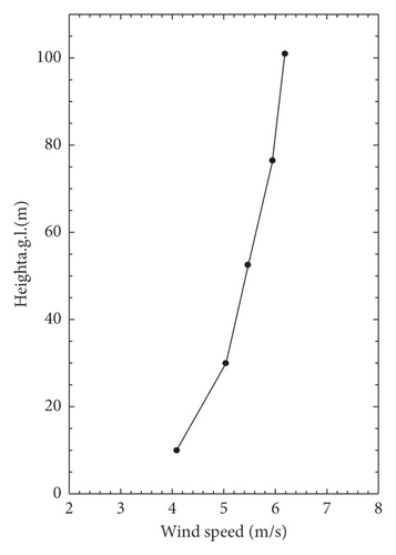
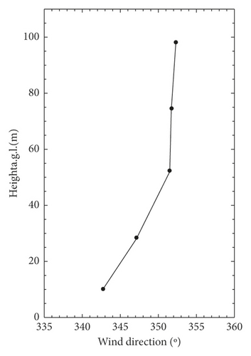
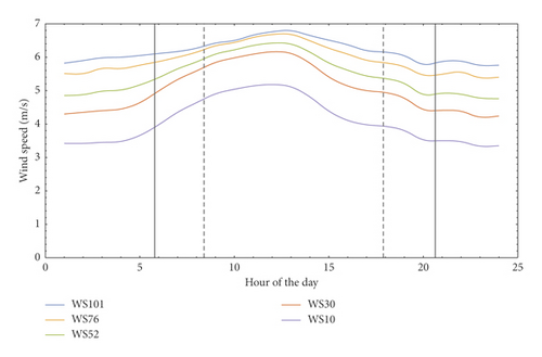
Monthly statistics of the top-mounted anemometer, WS101, show high wind speeds during the fall and winter periods, while the averaged wind speeds get lower in the summer and spring as expected due to the local weather conditions (Table 3). Wind data were split into 12 equal wind direction sectors, based on the vane measurements at 98 m coupled with the top-mounted cup anemometer at 101 m. Directional wind speed statistics when the top-mounted anemometer is coupled with the closest wind vane at 98 m show highest energy density at sector 1 and sector 7, which are centered at 0^° and 180^°, respectively (Table 4).

Table 3. Monthly wind speed statistics (all in m/s) of the top-mounted cup anemometer, WS101.

Month	Recovery (%)	Mean	Median	Min	Max	Std. dev.
Jan	98.25	6.557	5.123	0.305	23.611	5.391
Feb	99.68	5.511	5.141	0.306	16.776	3.354
Mar	99.66	6.523	6.365	0.305	19.775	3.511
Apr	98.4	4.396	3.499	0.3	19.561	3.654
May	99.26	5.472	4.528	0.3	15.704	3.958
Jun	99.49	5.127	5.227	0.306	13.92	2.97
Jul	99.48	6.476	6.682	0.315	15.445	3.143
Aug	99.64	7.736	8.32	0.304	15.472	3.498
Sep	99.56	7.016	6.452	0.301	20.19	4.217
Oct	98.75	5.617	5.291	0.308	16.658	3.433
Nov	99.91	7.221	7.078	0.348	18.321	3.667
Dec	99.53	6.447	5.538	0.301	23.628	4.432

Total	99.3	6.185	5.825	0.3	23.628	3.933

Table 4. Directional wind speed statistics of the top-mounted cup anemometer, WS101, based on the closest wind vane, WD98.

Direction		Rec.	Fre.	Mean	Median	Min	Max	Std. dev.
Sector	Range	(%)	(%)	(m/s)	(m/s)	(m/s)	(m/s)	(m/s)
1	345°–15°	99.75	45.65	7.564	7.511	0.403	23.628	3.696
2	15°–45°	98.9	11.21	5.921	4.629	0.403	23.611	4.871
3	45°–75°	95.83	1.95	1.614	1.355	0.405	13.227	1.127
4	75°–105°	95.19	1.41	1.772	1.369	0.418	7.588	1.15
5	105°–135°	93.11	1.3	1.442	1.138	0.403	8.046	1.022
6	135°–165°	97.12	3.7	4.074	2.542	0.401	19.775	3.912
7	165°–195°	98.94	12.59	6.057	5.992	0.404	19.2	3.684
8	195°–225°	98.28	7.59	5.163	5.161	0.402	16.151	2.836
9	225°–255°	96.03	2.75	4.693	4.817	0.405	13.211	2.541
10	255°–285°	95.26	2.09	4.756	4.784	0.412	13.536	2.601
11	285°–315°	98.17	4.66	5.52	5.316	0.401	14.8	2.804
12	315°–345°	97.52	5.07	4.648	4.04	0.403	16.122	3.122

Total		98.71	100	6.22	5.857	0.401	23.628	3.919

3. Distribution Analysis

In the last decade, several other distribution functions have been put forward/have been proposed, among which the most commonly used in the literature seem to be the following: Rayleigh, Weibull, Lognormal, Gamma, Pearson, Kappa, Erlang, and Gumble or bimodals of these [13–17]. Among the referenced studies, the general conclusion is that the two- or three-parameter Weibull distribution is the best distribution function to describe the wind characteristics [11, 18]. This is also reflected in industry applications, where any major wind energy or wind field modeling tool employs the two-parameter Weibull function (e.g., WAsP and WindPRO).

In the current study, selected dataset is also used for analysis using sector wise Weibull distribution function. Two-parameter Weibull function is used with each dataset split with sector wise wind direction; each holds 30° sections. The relationship between the mean wind speed U and the Weibull parameters, similar to equation (1), is given in equation (5); A is the scale and k is the shape parameter as before. Mean value of the wind speed can be calculated. Power density, P_d, can also be computed from the third moment of the equation (see (6)). Gamma (Γ) is the Euler Gamma Function (equation (7)).

(5)

(6)

(7)

Several different methods have been studied extensively in the past by the wind energy community. A review of the literature shows a great variety of formulations in estimating the Weibull distribution parameters (Table 5). The literature includes Empirical Method (EM), Power Density Method (PDM), Graphical Method (GM), Maximum Likelihood Method (MLM), Modified (Weighted) Maximum Likelihood Method (MMLM), Moment Methods (MM), and Least Square Method (LSM). It is also observed that the Wind Atlas Analysis and Application Program (WAsP) (official website: http://www.WAsP.dk) method has a limited use in such studies. Most of the studies using the WAsP method through the WAsP software are not comparing it to other methods [34, 35], but see [36]. In the current study, a selection of methods from the literature was used for the estimation of Weibull parameters.. Elimination of methods is done through similarities. Between similar methods of EM and PDM and between GM and LSM, the EM and the LSM are chosen, respectively. Moment methodologies have similarities with WAsP; therefore they are ignored. Five methods are shortlisted for the study: EM, MLM, MMLM, LSM, and WAsP.

Table 5. Selected studies related to the estimation of Weibull distribution in the last 20 years and the estimation of Weibull parameter methods used. WAsP method is not fully explained and presented in literature, except the technical documents of the WAsP software.

Study	EM	PDM	GM	MLM	MMLM	MM	LSM
Garcia [19]			x	x	x
Seguro [20]			x	x	x
Donk [21]				x	x		x
Ramirez [22]				x		x	x
Carta [23]				x			x
Cellura [24]				x
Akdag [25]	x		x	x		x
Saleh [26]		x	x	x	x
Khahro [27]	x	x	x	x	x
Arslan [28]				x		x
Mohammadi [29]	x	x	x	x	x
Katinas [30]	x	x	x				x
Ali [31]		x
Kang [32]	x		x		x	x
Polnumtiang [33]			x

3.1. Empirical Method (EM)

One of the most well-known and simple methods for estimating the Weibull parameters is the Empirical Method (EM), derived from the power density function [25, 27, 29, 30, 32]. The energy factor can be calculated as the ratio between the mean of the sum of cubes of all wind speeds and the cube of the mean wind speed (equation (8)). After E_f is calculated, one can easily use a derived numerical solution of k and A (equation (9)). The simplicity of the equation makes it very useful for initial calculations, but it has also been observed that the fit is not as good as that in other methods when there is low wind speed and high turbulence, which makes the Weibull PDF not a smooth curve. Nevertheless, it was chosen for this study as a reference formulation in order to explore the possible differences with more advanced methods.

(8)

(9)

(10)

3.2. Maximum Likelihood Method (MLM)

Another well-known and widely used method is the Maximum Likelihood Method (MLM) [20–29]. In MLM, the k parameter is found with the iteration of equation (10) for n number of samples with the initial shape parameter with the value of k = 2. After finding k within the desired limits with equation (11), the scale parameter A can be computed with equation (12).

(11)

(12)

3.3. Modified Maximum Likelihood Method (MMLM)

There is an alternative version of MLM, which has a modification on the wind frequencies [20, 21, 26, 27, 30, 32]. The method is mostly preferred when there is a large amount of missing data. All wind frequency values are weighted based on the available data; therefore the method is called Modified Maximum Likelihood Method (MMLM) (sometimes it is also called Weighted Maximum Likelihood Method in literature). Equation (11) is rewritten with the addition of the frequency by knowing that all the samples are above 0 m/s (equation (13)). The same iteration from MLM is applied to calculate the modified scale parameter A_m as in equation (14).

(13)

(14)

3.4. Least Square Method (LSM)

A less preferred method but one that is known to be more accurate for diverse frequencies distributions is the Least Square Method (LSM) [21, 23, 30, 37]. The Weibull function is transformed into a linear function format as in “y = Gain · x + Offset.” In order to make this transition, log normal of both sides of equation (2) is taken and this leads to the desired format as in equation (15). The left side of the equation can be computed from the wind speed variable and a fit algorithm can be used to calculate k and A.

(15)

3.5. WAsP Weibull Method

This method uses a different approach for estimating the Weibull parameters; it assumes that the wind speed above the mean value is most likely to create the maximum power. Therefore, Weibull fitting by using only the data above the mean wind speed value is considered to be more realistic by the method’s developers [38]. Nevertheless, that does not mean it is more effective for diverse frequencies distributions; therefore it has been selected as one of the methods to be studied. The reference documentation about the method is not detailed but the WAsP method is one of the most used methodologies through the WAsP software family.

The first step in the method is to define a parameter that gives the probability of the wind speeds above the mean value, which can be calculated through the cumulative density function (CDF) with the Weibull parameters (equation (2)). If the mean wind speed is applied to the function, the cumulative density will be the total sum of the probabilities of the wind speeds below the mean values; therefore 1-F (U) becomes the proportion of the values above the mean value, U_p (equation (16)).

(16)

When both sides of the equation are taken as logarithmic normal (equation (17)), one can write the parameter A as a function of k or vice versa and calculate both in two steps. The shape parameter A can be written as a function of k through the power density function (equation (6)), which is equal to the mean of cube sum of wind speed samples (equation (18)). If parameter A is singled out, it can be written as a function of k(equation (19)). If equations (17) and (19) are merged as in equation (20), one can use iterative numerical steps to solve k and place the result in equation (19) to calculate A.

(17)

(18)

(19)

(20)

Omnidirectional data and grouped sectors were used in the analysis (see Table 2). Sectors were grouped based on the common roughness and obstacle types of the sectors. Group I includes sectors 1 and 2, with the northerly winds and the highest number of samples. The urban area located in sectors 3, 4, and 5 constitutes Group II, which has the lowest number of samples and a total energy density calculated to be close to zero. Therefore, the results for Group II might be misleading; nevertheless they are still presented for the sake of completeness. The university zone, sectors 7 and 8, constitutes Group III and the sectors covered with hills from 8 to 12 form Group IV. The collected data were analyzed by wind speed bins of 0.5 m/s and all available data for the selected sectors were processed for the calculation.

4. Results

In order to understand the accuracy of the Weibull estimation method, most of the studies address the question as a statistical error and calculate the root mean square error (RMSE) based on the measured data.

(21)

where y_i is the measured value and x_i is the Weibull-parameters-based calculated value. However, this method can be misleading because it places the same importance on every range of wind speed and the total sum of errors is not weighted by the possible energy density. Therefore, in the current study, the accuracy is also evaluated through the power density function because this is the real effective difference between estimation methods when it comes to calculating the wind energy production. It is common to calculate the power density based on two datasets as in equation (22), where ρ is the air density and f_m is the frequency for the given wind speed range. The values can be used to drive an error percentage value, ε (equation (23)), compared to the measured value.

(22)

(23)

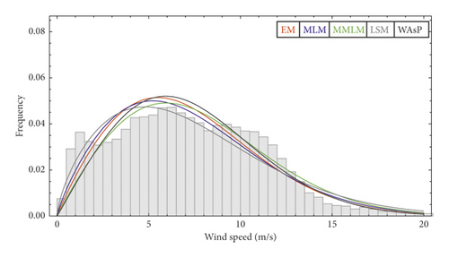
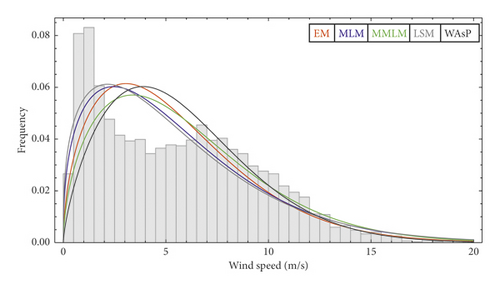
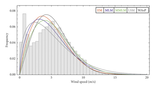
The omnidirectional results (Figure 4 and Table 6) show a minor error in power density prediction, as low as ± 3-4% for the methods EM, MLM, and WAsP, which is already within the limits of statistical uncertainty [39], while frequency levels show that almost 25% of the whole data is below 3 m/s, which is the cut-in wind speed for most turbines. When the sector wise results are observed (Figures 5–7 and Table 6), it is also seen that low wind speeds below 3-4 m/s are common and can affect the calculations for the all groups. Among the compared methods, MLM appears to be the best performing overall, with a maximum error of 3% in power density calculations at the sectors without urban areas. The WAsP gives the second lowest percentage error, arriving at similar results to those of EM, with the difference being that the WAsP method has a better fit for wind speeds close to the mean level, which is intentional by the design of the methodology, as was described in subsection “WAsP Weibull Method.” MMLM and LSM produce high error percentages nearly in every sector and even in the omnidirectional fit. RMSE and R² values show an inverse relationship as is expected. When the RMSE increases, the R² parameter decreases, and vice versa, but there is no clear relationship between these statistical measures and the calculated power density estimation errors.

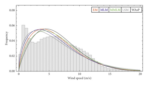
Table 6. Comparison results from four different groups.

Sector	Power density measured (W/m²)	Method	k	A (m/s)	RMSE [10⁻³]	R² (%)	Power density fitted (W/m²)
All	341	EM	1.64	6.9	3.16	84.80	327
		MLM	1.53	6.8	2.93	86.20	350
		MMLM	1.68	7.3	3.08	83.80	381
		LSM	1.42	6.9	2.79	86.40	394
		WAsP	1.79	7.2	3.49	81.70	330

1-2	460	EM	1.91	8.1	2.23	91.00	444
		MLM	1.82	8.1	2.19	90.80	460
		MMLM	1.95	8.6	2.07	91.50	505
		LSM	1.68	8.2	2.21	89.30	513
		WAsP	2.02	8.3	2.3	90.80	448

6-7	275	EM	1.53	6.1	5.03	66.30	252
		MLM	1.39	6.1	4.51	71.60	269
		MMLM	1.55	6.6	5.04	60.50	296
		LSM	1.34	6	4.36	72.80	279
		WAsP	1.71	6.5	5.82	54.40	260

8–12	155	EM	1.82	5.5	5.62	71.80	146
		MLM	1.63	5.5	5.33	71.50	158
		MMLM	1.85	6	5.21	71.20	179
		LSM	1.42	5.6	5.19	67.00	188
		WAsP	2.06	5.8	5.95	70.60	149

5. Conclusion

Yearly 10-minute statistics from a 101 m met. Mast and top-mounted cup anemometer data have been used for comparison of Weibull parameter estimation. The measurement period is from 27 December 2017 to 27 December 2018 for a total of 1 full year with over 99% recovery rate. The data has almost 25% low wind speeds, which causes difficulties on the estimation, which is the core reason of the study. Vertical wind characteristics from the met. mast show that the measurement location has wind shear within limits of the standards and vertical directional turn is negligible between cup anemometer and the vane used in the study. Basic statistics of monthly and 12 equal wind sectors are calculated. Sectors 2 to 6 are excluded from the study due to the low recovery rate and urban areas closer than 500 m. The results leading to the conclusion are made with the other sectors.

The omnidirectional and sector wise calculations for five different estimation methods are tested and the results are presented with observed statistics. The distribution fits are analyzed through root mean square errors (RMSE) and R² parameters in addition to the power density error function (ε). The results show that the Maximum Likelihood method (MLM) has the best performance. A clear link has not been found between ε and RMSE and/or R² contrary to the several previously cited studies, where conclusions are made based on these statistical parameters. Other estimation methods show high uncertainty and power density calculation error. These two results lead to the fact that power density error estimation is the most effective way of checking the distribution fit quality even though similar studies. Based on Group III results, it can be said that the low number of samples with low wind speeds causes high uncertainty and deviation in any method.

Several wind data analysis tools in the world use WAsP Weibull fitting method as the core estimation method for Weibull parameters through the WAsP software. Nevertheless, it is observed that, for the diverse winds, Maximum Likelihood Method is much more stable and has a better correlation with measured data. One should create observational wind statistical data by means of MLM and apply the Weibull parameters to the model even if the used model is WAsP software.

In this study, wind speed data in the form of 10-minute statistics from a 101 m met. mast with top-mounted cup anemometers are used to compare different methods for the estimation of Weibull parameters. The measurement period was from 27 December 2017 to 27 December 2018, that is, one full year of data with over 99% recovery rate. A high proportion of the dataset (over 20%) consisted of low wind speeds, which are known to cause difficulties in the parameter estimation, and this is the main driver that motivated the study. The vertical wind characteristics from the met. mast show that the measurement location has wind shear within the limits of the industry standards. Basic statistics of monthly and 12 equal wind sectors were calculated. The sectors are divided into four groups (Figure 1). The results leading to the conclusion were produced with data from these groups. Nevertheless, Group II does not have enough amount of data to compare and present the methods; therefore, it is excluded from the results.

The omnidirectional and sector wise calculations for five different estimation methods were tested and the results are presented with the observed statistics. The distribution fits were analyzed through root mean square errors (RMSE) and R² parameters in addition to the power density error function (ε). The results show that the Maximum Likelihood method (MLM) had the best performance for the dataset. A clear link has not been found between ε and RMSE and/or R² contrary to several previous studies, where conclusions on performance were made based on these statistical parameters. Selected list of these referenced studies is in Table 5. The other estimation methods tested showed high uncertainty and higher power density calculation errors. These two results lead to the conclusion that power density error estimation is the most effective way of checking the distribution fit quality of an estimation method even though similar studies only focus on the statistical terms of RMSE and/or R². Based on the results of Group III, it is evident that low number of samples combined with low wind speeds causes high uncertainty and deviation in any method.

Several wind data analysis tools in the world use the WAsP Weibull fitting method as the core estimation method for Weibull parameters through the WAsP software. Nevertheless, it is demonstrated that, in the case of diverse winds, the Maximum Likelihood Method is much more stable and has a better correlation with measured data. For these types of datasets, it is advisable to create observational wind statistical data by means of MLM and apply the Weibull parameters to the model.

Conflicts of Interest

The author declares that there are no conflicts of interest regarding the publication of this article.

Acknowledgments

This project has been supported by the Scientific and Technological Research Council of Turkey (TÜBİTAK) (Grant no. 215M384).

Open Research

Data Availability

The data used to support the findings of this study are available from the corresponding author upon request.

References

1 IEC, Wind Turbines-Part 1: Design Requirements (IEC standart 61400-1), 2005, 3rd edition, IEC, Geneva, Switzerland.
Google Scholar
2 MEASNET, Evaluation of Site-specific Site Conditions, 2016, MEASNET, Madrid, Spain.
Google Scholar
3 Bingöl F., Mann J., and Foussekis D., Conically scanning lidar error in complex terrain, Meteorologische Zeitschrift. (2009) 18, no. 2, 189–195, https://doi.org/10.1127/0941-2948/2009/0368, 2-s2.0-68249152257.
10.1127/0941-2948/2009/0368
Web of Science® Google Scholar
4 Bradley S., Perrott Y., Behrens P., and Oldroyd A., Corrections for wind-speed errors from sodar and lidar in complex terrain, Boundary-Layer Meteorology. (2012) 143, no. 1, 37–48, https://doi.org/10.1007/s10546-012-9702-0, 2-s2.0-84857993993.
10.1007/s10546-012-9702-0
Web of Science® Google Scholar
5 Vasiljevia N., José M., Palma L. M. et al., Methodology for atmospheric multi-doppler lidar experiments, Atmospheric Measurement Techniques. (2017) 10, no. 9, 3463–3483, https://doi.org/10.5194/amt-10-3463-2017, 2-s2.0-85029953871.
10.5194/amt-10-3463-2017
Web of Science® Google Scholar
6 Mann J., Menke R., Vasiljević N., Berg J., and Troldborg N., Challenges in using scanning lidars to estimate wind resources in complex terrain, The Science of Making Torque from Wind 2018 - Politecnico di Milano (POLIMI). (2018) 1037, 072017, https://doi.org/10.1088/1742-6596/1037/7/072017, 2-s2.0-85049677283.
10.1088/1742-6596/1037/7/072017
Google Scholar
7 Jamil M., Parsa S., and Majidi M., Wind power statistics and an evaluation of wind energy density, Renewable Energy. (1995) 6, no. 5-6, 623–628, https://doi.org/10.1016/0960-1481(95)00041-h, 2-s2.0-0029137421.
10.1016/0960-1481(95)00041-H
Web of Science® Google Scholar
8 Mathew S., Pandey K. P., and Kumar.V A., Analysis of wind regimes for energy estimation, Renewable Energy. (2002) 25, no. 3, 381–399, https://doi.org/10.1016/s0960-1481(01)00063-5, 2-s2.0-0036488890.
10.1016/S0960-1481(01)00063-5
Web of Science® Google Scholar
9 Luna R. E. and Church H. W., Estimation of long-term concentrations using a “universal” wind speed distribution, Journal of Applied Meteorology. (1974) 13, no. 8, 910–916, https://doi.org/10.1175/1520-0450(1974)013<0910:eoltcu>2.0.co;2.
10.1175/1520-0450(1974)013<0910:EOLTCU>2.0.CO;2
Web of Science® Google Scholar
10 Troen I. B. and Petersen E. L., European Wind Atlas, 1989, Risø National Laboratory, Roskilde, Denmark.
Google Scholar
11 Stewart D. A. and Essenwanger O. M., Frequency distribution of wind speed near the surface, Journal of Applied Meteorology. (1978) 17, no. 11, 1633–1642, https://doi.org/10.1175/1520-0450(1978)017<1633:fdowsn>2.0.co;2.
10.1175/1520-0450(1978)017<1633:FDOWSN>2.0.CO;2
Web of Science® Google Scholar
12 Deaves D. M. and Lines I. G., On the fitting of low mean windspeed data to the weibull distribution, Journal of Wind Engineering and Industrial Aerodynamics. (1997) 66, no. 3, 169–178, https://doi.org/10.1016/s0167-6105(97)00013-5, 2-s2.0-0031086905.
10.1016/S0167-6105(97)00013-5
Web of Science® Google Scholar
13 Zhou J., Erdem E., Li G., and Shi J., Comprehensive evaluation of wind speed distribution models: a case study for North Dakota sites, Energy Conversion and Management. JUL 2010, 51, no. 7, 1449–1458, https://doi.org/10.1016/j.enconman.2010.01.020, 2-s2.0-77949652893.
10.1016/j.enconman.2010.01.020
Web of Science® Google Scholar
14 Morgan E. C., Lackner M., Vogel R. M., and Baise L. G., Probability distributions for offshore wind speeds, Energy Conversion and Management. JAN 2011, 52, no. 1, 15–26, https://doi.org/10.1016/j.enconman.2010.06.015, 2-s2.0-78049503716.
10.1016/j.enconman.2010.06.015
Web of Science® Google Scholar
15 Chang T.P., Estimation of wind energy potential using different probability density functions, Applied Energy. (2011) 88, no. 5, 1848–1856, https://doi.org/10.1016/j.apenergy.2010.11.010, 2-s2.0-79551525027.
10.1016/j.apenergy.2010.11.010
Web of Science® Google Scholar
16 Ouarda T. B. M. J., Charron C., Shin J. Y. et al., Hosary. Probability distributions of wind speed in the UAE, Energy Conversion and Management. (2015) 93, 414–434, https://doi.org/10.1016/j.enconman.2015.01.036, 2-s2.0-84922278881.
10.1016/j.enconman.2015.01.036
Web of Science® Google Scholar
17 Wais P., A review of Weibull functions in wind sector, Renewable and Sustainable Energy Reviews. (2017) 70, 1099–1107, https://doi.org/10.1016/j.rser.2016.12.014, 2-s2.0-85008395741.
10.1016/j.rser.2016.12.014
Web of Science® Google Scholar
18 Conradsen K., Nielsen L. B., and Prahm L. P., Review of weibull statistics for estimation of wind speed distributions, Journal of Climate and Applied Meteorology. (1984) 23, no. 8, 1173–1183, https://doi.org/10.1175/1520-0450(1984)023<1173:rowsfe>2.0.co;2.
10.1175/1520-0450(1984)023<1173:ROWSFE>2.0.CO;2
Web of Science® Google Scholar
19 Garcia A., Torres J. L., Prieto E., and De Francisco A., Fitting wind speed distributions: a case study, Solar Energy. (1998) 62, no. 2, 139–144, https://doi.org/10.1016/s0038-092x(97)00116-3, 2-s2.0-0032006463.
10.1016/S0038-092X(97)00116-3
Web of Science® Google Scholar
20 Seguro J. V. and Lambert T. W., Modern estimation of the parameters of the Weibull wind speed distribution for wind energy analysis, Journal of Wind Engineering and Industrial Aerodynamics. (2000) 85, no. 1, 75–84, https://doi.org/10.1016/s0167-6105(99)00122-1, 2-s2.0-0034161613.
10.1016/S0167-6105(99)00122-1
Web of Science® Google Scholar
21 van Donk S. J., Wagner L. E., Skidmore E. L., and Tatarko J., Comparison of the weibull model with measured wind speed distributions for stochastic wind generation, Transactions of the ASAE. (2005) 48, 2, 503510, https://doi.org/10.13031/2013.18324.
10.13031/2013.18324
Google Scholar
22 Ramirez P. and Carta J. A., The use of wind probability distributions derived from the maximum entropy principle in the analysis of wind energy. A case study, Energy Conversion and Management. (2006) 47, no. 15-16, 2564–2577, https://doi.org/10.1016/j.enconman.2005.10.027, 2-s2.0-33646754223.
10.1016/j.enconman.2005.10.027
Web of Science® Google Scholar
23 Carta J. A. and Ramírez P., Analysis of two-component mixture Weibull statistics for estimation of wind speed distributions, Renewable Energy. MAR 2007, 32, no. 3, 518–531, https://doi.org/10.1016/j.renene.2006.05.005, 2-s2.0-33748503142.
10.1016/j.renene.2006.05.005
Web of Science® Google Scholar
24 Cellura M., Cirrincione G., Marvuglia A., and Miraoui A., Wind speed spatial estimation for energy planning in Sicily: a neural kriging application, Renewable Energy. (2008) 33, no. 6, 1251–1266, https://doi.org/10.1016/j.renene.2007.08.013, 2-s2.0-39349083955.
10.1016/j.renene.2007.08.013
Web of Science® Google Scholar
25 Akdag S. A. and Ali D., A new method to estimate weibull parameters for wind energy applications, Energy Conversion and Management. JUL 2009, 50, no. 7, 1761–1766, https://doi.org/10.1016/j.enconman.2009.03.020, 2-s2.0-67349247564.
10.1016/j.enconman.2009.03.020
Web of Science® Google Scholar
26 Saleh H., Azm Aly A. A. E., and Hady S. A.-, Assessment of different methods used to estimate Weibull distribution parameters for wind speed in zafarana wind farm, Suez Gulf, Egypt, Energy. (2012) 44, no. 1, 710–719, https://doi.org/10.1016/j.energy.2012.05.021, 2-s2.0-84864325860.
10.1016/j.energy.2012.05.021
Web of Science® Google Scholar
27 Khahro S. F., Tabbassum K., Mahmood Soomro A., Dong L., and Liao X., Evaluation of wind power production prospective and Weibull parameter estimation methods for Babaurband, Sindh Pakistan, Energy Conversion and Management. (2014) 78, 956–967, https://doi.org/10.1016/j.enconman.2013.06.062, 2-s2.0-84892965166.
10.1016/j.enconman.2013.06.062
Web of Science® Google Scholar
28 Arslan T., Bulut Y. M., and Altın Yavuz A., Comparative study of numerical methods for determining Weibull parameters for wind energy potential, Renewable and Sustainable Energy Reviews. (2014) 40, 820–825, https://doi.org/10.1016/j.rser.2014.08.009, 2-s2.0-84906668609.
10.1016/j.rser.2014.08.009
Web of Science® Google Scholar
29 Mohammadi K., Alavi O., Ali M., Goudarzi N., and Jalilvand M., Assessing different parameters estimation methods of Weibull distribution to compute wind power density, Energy Conversion and Management. (2016) 108, 322–335, https://doi.org/10.1016/j.enconman.2015.11.015, 2-s2.0-84947969727.
10.1016/j.enconman.2015.11.015
ADS Web of Science® Google Scholar
30 Katinas V., Marčiukaitis M., Gecevičius G., and Markevičius A., Statistical analysis of wind characteristics based on weibull methods for estimation of power generation in Lithuania, Renewable Energy. (2017) 113, 190–201, https://doi.org/10.1016/j.renene.2017.05.071, 2-s2.0-85020042157.
10.1016/j.renene.2017.05.071
Web of Science® Google Scholar
31 Ali S., Lee S.-M., and Jang C.-M., Statistical analysis of wind characteristics using Weibull and Rayleigh distributions in Deokjeok-do Island-incheon, South Korea, Renewable Energy. (2018) 123, 652–663, https://doi.org/10.1016/j.renene.2018.02.087, 2-s2.0-85042454783.
10.1016/j.renene.2018.02.087
Web of Science® Google Scholar
32 Kang D., Ko K., and Huh J., Comparative study of different methods for estimating weibull parameters: a case study on Jeju island, South Korea, Energies. (2018) 11, no. 2, https://doi.org/10.3390/en11020356, 2-s2.0-85054861425.
10.3390/en11020356
Web of Science® Google Scholar
33 Polnumtiang S. and Tangchaichit K., Wind speed and power characteristics of Kalasin province, Thailand, IOP Conference Series: Earth and Environmental Science. (2018) 150, 012020, https://doi.org/10.1088/1755-1315/150/1/012020, 2-s2.0-85048446863.
10.1088/1755-1315/150/1/012020
Google Scholar
34 Prahm B., Vihma T., Atlaskin E. et al., Production of the finnish wind atlas, Wind Energy. (2013) 16, no. 1, 19–35, https://doi.org/10.1002/we.517, 2-s2.0-84872937939.
10.1002/we.517
Web of Science® Google Scholar
35 Nawri N., Petersen G. N., Bjornsson H. et al., The wind energy potential of Iceland, Renewable Energy. (2014) 69, 290–299, https://doi.org/10.1016/j.renene.2014.03.040, 2-s2.0-84898830088.
10.1016/j.renene.2014.03.040
Web of Science® Google Scholar
36 Jourdier B. and Philippe D., Errors in wind resource and energy yield assessments based on the weibull distribution, Annales Geophysicae. (2017) 35, no. 3, 691–700, https://doi.org/10.5194/angeo-35-691-2017, 2-s2.0-85020002270.
10.5194/angeo-35-691-2017
Web of Science® Google Scholar
37 Ramirez P. and Carta J. A., Influence of the data sampling interval in the estimation of the parameters of the Weibull wind speed probability density distribution: a case study, Energy Conversion and Management. (2005) 46, no. 15-16, 2419–2438, https://doi.org/10.1016/j.enconman.2004.11.004, 2-s2.0-17744370511.
10.1016/j.enconman.2004.11.004
Web of Science® Google Scholar
38 WAsP 12 Documentation, Last Edited 2018-06-01, 2018, Department of Wind Energy, Technical University of Denmark (DTU), Roskilde, Denmark.
Google Scholar
39 Kwon S.-D., Uncertainty analysis of wind energy potential assessment, Applied Energy. (2010) 87, no. 3, 856–865, https://doi.org/10.1016/j.apenergy.2009.08.038, 2-s2.0-71849115521.
10.1016/j.apenergy.2009.08.038
Web of Science® Google Scholar

Citing Literature

All articles

Comparison of Weibull Estimation Methods for Diverse Winds

Abstract

1. Introduction

2. Experimental Setup and General Wind Characteristics