Volume 2019, Issue 1 9275051
Research Article
Open Access

Analysis of a Stochastic SIR Model with Vaccination and Nonlinear Incidence Rate

Amine El Koufi

Corresponding Author

Amine El Koufi

Laboratory of Analysis Modeling and Simulation (LAMS), Faculty of Sciences Ben M’sik, Hassan II University, P.O. Box 7955, Sidi Othman, Casablanca, Morocco uh2c.ac.ma

Search for more papers by this author
Jihad Adnani

Jihad Adnani

Laboratory of Analysis Modeling and Simulation (LAMS), Faculty of Sciences Ben M’sik, Hassan II University, P.O. Box 7955, Sidi Othman, Casablanca, Morocco uh2c.ac.ma

Search for more papers by this author
Abdelkrim Bennar

Abdelkrim Bennar

Laboratory of Analysis Modeling and Simulation (LAMS), Faculty of Sciences Ben M’sik, Hassan II University, P.O. Box 7955, Sidi Othman, Casablanca, Morocco uh2c.ac.ma

Search for more papers by this author
Noura Yousfi

Noura Yousfi

Laboratory of Analysis Modeling and Simulation (LAMS), Faculty of Sciences Ben M’sik, Hassan II University, P.O. Box 7955, Sidi Othman, Casablanca, Morocco uh2c.ac.ma

Search for more papers by this author
First published: 21 August 2019
Citations: 17
Academic Editor: Elena Kaikina

Abstract

We expand an SIR epidemic model with vertical and nonlinear incidence rates from a deterministic frame to a stochastic one. The existence of a positive global analytical solution of the proposed stochastic model is shown, and conditions for the extinction and persistence of the disease are established. The presented results are demonstrated by numerical simulations.

1. Introduction

Mathematical models play an important role in the analysis and control of infectious diseases, and thus effective measures can be taken to reduce its transmission as much as possible. The study of mathematical models in epidemiology has received much attention from many scientists, and some novel results are obtained [14]. Recently, stochastic analysis has widely been applied in mathematical modeling in biology [59].

For compartmental mathematical models, the total population is divided into three classes, namely, susceptible population S(t), infected population I(t), and recover population R(t). For more details, see [10]. For some diseases, such as AIDS, rubella, varicella, hepatitis B, hepatitis, syphilis, and mumps, it is one of the main transmission modes that infected mothers infect their unborn or newborn offsprings, called vertical transmission [11]. Meng and Chen [12] proposed an SIR epidemic model with vaccination and vertical transmission mode as follows:
()
where b is the mortality rate in the susceptible and the recovered individuals and d is the mortality rate in the infective individuals. The constants p and q (p + q = 1) are vertical transmission rates, namely, p and q are, respectively, the proportion of the offspring of infective parents that are susceptible individuals and the rest are born infected. The arrival of newborns constitutes a recruitment rate of b(S + R) into the susceptible individuals and qdI into the infectious individuals. m(0 ≤ m ≤ 1) is the successful vaccination proportion to the newborn from S and R, r is the recover rate in the infective individuals into recovered individuals, and β is the contact rate. System (1) has a basic reproduction number R0 defined by
()
On the contrary, environmental fluctuations have great influence on all aspects of real life. The aim of this work is to study the effect of these environmental fluctuations on the transmission rate β. We assume that the stochastic perturbations are of white noise type, that is, , where B(t) is a Brownian motion and σ is the intensity. Then, the stochastic version corresponding to the deterministic model (1) with general incidence rate is as follows:
()
where B(t) is the independent standard Brownian motions defined on a complete probability space with a filtration satisfying the usual conditions (i.e., it is increasing and right continuous while 0 contains all P null sets).
g(S, I) = βSI/(1 + α1S + α2I + α3SI) is the incidence rate, where α1, α2, α3 ≥ 0. In addition, the incidence rate is the number of new infected situations by population in a determined time period. To model the disease transmission process, several authors employ the following bilinear incidence rate βSI, where β is a positive constant [13]. Yet, there exist many forms of nonlinear incidence rate and every form presents some advantages [1416]. It is very important to note that g(S, I) = βSI/(1 + α1S + α2I + α3SI) is a general form which represents mutual interference between S and I. in particular cases:
  • (1)

    If α1 = α2 = α3 = 0, g(S, I) becomes a bilinear incidence rate

  • (2)

    If α1 = α2 = 0 or α1 = α3 = 0, g(S, I) becomes a saturated incidence rate [17]

  • (3)

    If α3 = 0, g(S, I) becomes a Beddington–DeAngelis functional response [18]

  • (4)

    If α3 = α1α2, g(S, I) becomes the Crowley–Martin functional response presented in [19]

Next, we consider the d-dimensional stochastic system:
()
where f(x, t) is a function in IRd defined in [t0, +) and g(x, t) is a d × m matrix, and f and g are locally Lipschitz functions in x. {B(t)}t≥0 is a d-dimensional standard Wiener process defined on the above probability space.
Denote by the family of all nonnegative functions U(x, t) defined on IRd × [t0, +) such that they are continuously twice differentiable in x and once in t. The differential operator [16] associated with (4) is defined by
()
If the differential operator acts on a function , then
()
where Ut(x, t) = U/t, Ux(x, t) = (U/x1, …, U/xd), and Uxx(x, t) = (2U/xixj).

The organization of this paper is as follows. In Section 2, we show the existence of unique positive global solution to the given SDE system. Extinction and persistence in mean results are explored in Section 3 and Section 4, respectively. In Section 5, the analytical results are illustrated with the support of numerical examples. Finally, we close the paper with conclusion and future directions.

2. Existence and Uniqueness of the Nonnegative Solution

As we are dealing with the population model, the positive solution of the model is of our interest. The coefficients of (3) are locally Lipschitz continuous and do not satisfy the linear growth condition, so the solution of (3) may explode at a finite time. The following theorem shows that the solution is positive and will not explode at a finite time.

We define a subset Δ of IR3 as follows:
()

Theorem 1. For any given initial value X0 = (S(0), I(0), R(0)) ∈  Δ, there is a unique positive solution X(t) = (S(t), I(t), R(t)) of (3) on t ≥ 0, and the solution will remain in Δ with probability 1, namely, (S(t), I(t), R(t)) ∈  Δ for all t ≥ 0 almost surely (briefly a.s.).

Proof 1. Since the coefficients of system (3) are locally Lipschitz continuous, for any initial value (S(0), I(0), R(0)) ∈  Δ, there is a unique local solution on [0, τe), where τe is the explosion time. To show this solution is global, we need to show that τe =  a.s. For this, we define the stopping time τ by

()
with the traditional setting inf ∅ = (as usual ∅ denotes the empty set). We have ττe. If we can show that τ = a.s., then τe = a.s. and (S(t), I(t), R(t)) ∈  Δ for all t ≥ 0. In other words, to complete the proof, all we only need to show is that τ = . Assume that this statement is false, then there exists a T > 0 such that P(τ < T) > 0. Define a function U, by the expression
()

Using Itô’s formula, we get

()

Since f(S, I) ≥ 1, and S ≤ 1, I ≤ 1, we get,

()
where H = β + 2b + pd + r + σ2. Then, we have
()

Note that some components of X(τ) equal 0; thus, limtτU(X(t)) = +.

Letting tτ in (12), we obtain

()
which contradicts our assumption. Then, τ = a.s. This completes the proof of theorem.

3. Extinction

In the following, we give a condition for the extinction of the disease. Let
()

Theorem 2. Let (S(t), I(t), R(t)) be the solution of system (3) with initial value (S(0), I(0), R(0)) ∈  Δ. Assume that

  • (i)

    σ2 > β2/(2(pd + r)) or

  • (ii)

    Rs < 1 and σ2 < β

Then,

()

Namely, I(t) tends to zero exponentially a.s., i.e., the disease dies out with probability 1.

Proof 2. Applying Itô’s formula to system (3) leads to

()

Integrating both sides of (16) from 0 to t, we get

()
where , which is a local continuous martingale, and M(0) = 0. Moreover, its quadratic variation is
()

By the large number theorem for martingales [21], we obtain

()

If condition (i) is satisfied, dividing by t and taking the limit superior of both sides of (17), we get

()

If the condition (ii) is satisfied, note that

()

It follows that

()

Taking the superior limit of both sides of (22), we obtain

()
which implies that limt⟶+I(t) = 0.

Remark 1. From Theorem 1, we can get that the disease will die out if Rs < 1, and the white noise is not large such that σ2 < β, while if the white noise is large enough such that condition (i) is satisfied, then the infectious disease of system (3) goes to extinction almost surely.

4. Persistence

Here, we investigate the condition for the persistence of the disease. The basic reproduction number R0(see [20]), is the threshold between disease extinction and persistence, with extinction for R0 ≤ 1 and persistence for R0 > 1 in the deterministic model. In the stochastic model, we define the threshold of persistence for disease as
()

Definition 1. System (3) is said to be persistent in the mean if

()

We define

()

Theorem 3. If then the solution (S(t), I(t), R(t)) of system (3) with initial initial value (S(0), I(0), R(0)) ∈  Δ is persistent in mean. Moreover, we have

()
where χ = β(1 − m)(((r + dmp)/b)(1 − m) + ((α2 + α3)(pd + r)/β(1 − m))).

Proof 3. We have

()

Integrating from 0 to t and dividing by t > 0 the third equation of system (3), we get

()

From (28), one can get

()
where φ(t) = (R(t) − R(0))/t. From Itô’s formula and (3), we obtain
()

Integrating from 0 to t and dividing by t > 0 on both sides of yields

()

We can rewrite the inequality (32) as

()
where χ = β(1 − m)((r + dmp/b) − 1 + m + ((α2 + α3)(pd +  r)/β(1 − m))). We can see that R(t) ≤ 1 and I(t) ≤ 1. Thus, one has limt⟶+R(t)/t = 0, limt⟶+I(t)/t = 0, and limt⟶+φ(t) = 0. Taking the inferior limit of both sides of (33) yields
()

This completes the proof of theorem.

5. Numerical Simulations

In order to illustrate our theoretical results, we give some numerical simulations. The values of m, σ, and β will be varied over the different examples.

Example 1. We choose the parameters in system (3) as follows:

()

By calculation, we have R0 = 0.4902; in this case, the disease dies out as shown in Figure 1(a). By choosing m = 0.3, we obtain R0 = 1.635, and we deduce that the disease persists in the population. Figure 1(b) illustrates this result.
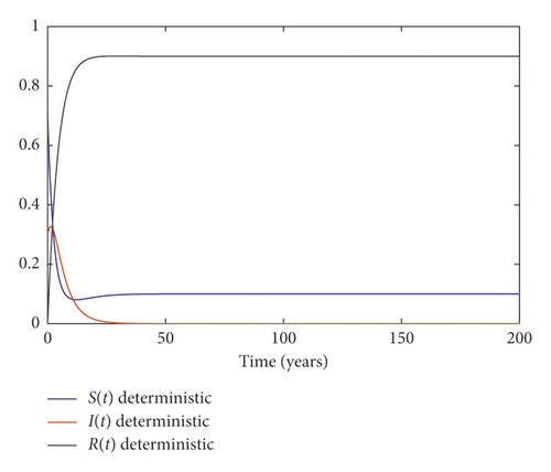
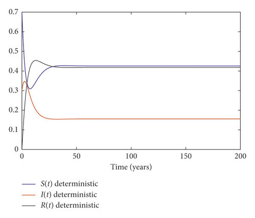
Details are in the caption following the image
Simulations of the path S(t), I(t), and R(t) for the corresponding deterministic system (1).
Details are in the caption following the image
Simulations of the path S(t), I(t), and R(t) for the corresponding deterministic system (1).

Example 2. We choose the parameters in system (3) as follows:

()

A simple computation shows that

()

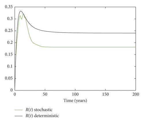
It follows that the condition of Theorem 2 is satisfied. We conclude that the disease dies out; Figure 2 illustrates this result.
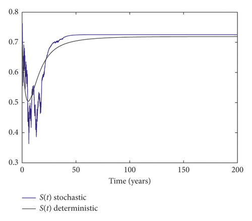
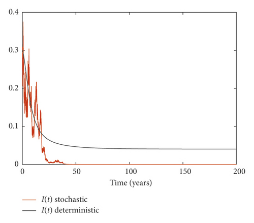
Details are in the caption following the image
Simulations of the path (a) S(t), (b) I(t), and (c) R(t) for the deterministic system (1) and the corresponding stochastic system (3).
Details are in the caption following the image
Simulations of the path (a) S(t), (b) I(t), and (c) R(t) for the deterministic system (1) and the corresponding stochastic system (3).
Details are in the caption following the image
Simulations of the path (a) S(t), (b) I(t), and (c) R(t) for the deterministic system (1) and the corresponding stochastic system (3).

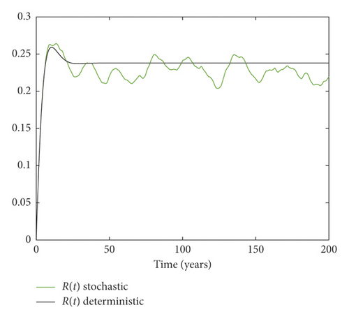
Example 3. On the contrary, we choose m = 0.05 and σ = 0.1 by simple calculation, and it can be found that which implies that the disease persists (Figure 3).
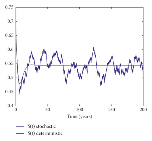
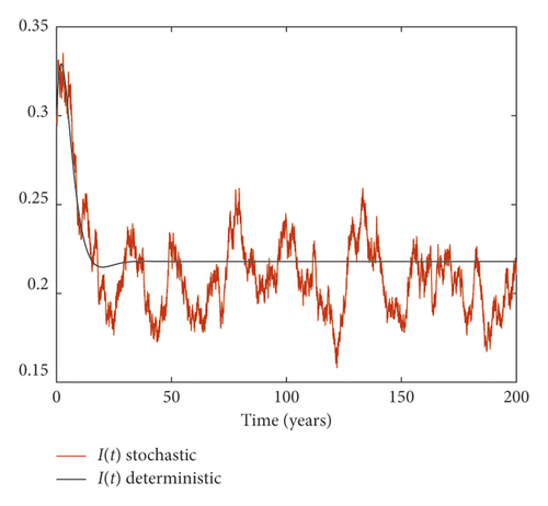
Details are in the caption following the image
Simulations of the path (a) S(t), (b) I(t), and (c) R(t) for the deterministic system (1) and the corresponding stochastic system (3).
Details are in the caption following the image
Simulations of the path (a) S(t), (b) I(t), and (c) R(t) for the deterministic system (1) and the corresponding stochastic system (3).
Details are in the caption following the image
Simulations of the path (a) S(t), (b) I(t), and (c) R(t) for the deterministic system (1) and the corresponding stochastic system (3).

6. Conclusion

This article discusses a stochastic SIR epidemic model with vertical transmission and vaccination and nonlinear incidence rate. We have shown that when the noise is so small such that σ2 < β, the extinction of the disease can be determined by the value of Rs, i.e., if Rs < 1, the disease dies out. Moreover, the disease dies out when the white noise is large enough such that σ2 > (β2/2(pd + r)).

The persistence of the disease is determined by , i.e., if , the disease persists. We presented some numerical simulations to illustrate the obtained analytical results. To go further in this study, we can give a new dimension to the stochastic SIR epidemic model (3) by introducing a different type of noise which is the random telegraph noise (RTN), modeled by the Markov chain. We will investigate this case in our future works.

Conflicts of Interest

The authors declare that there are no conflicts of interest regarding the publication of this paper.

Data Availability

The data used to support the findings of this study are available from the corresponding author upon request.

    The full text of this article hosted at iucr.org is unavailable due to technical difficulties.