Accurate degradation state recognition of rolling bearing is critical to effective condition based on maintenance for improving reliability and safety. In this work, a new architecture is proposed to recognize the degradation state of the rolling bearing. Firstly, the time-domain features including RMS, kurtosis, skewness and RMSEE, and Mel-frequency cepstral coefficients features are extracted from bearing vibration signals, which are then used as the input of k-means algorithm. These unlabeled features are clustered by k-means in order to define the different categories of the bearing degradation state. In this way, the original vibration signals can be labeled. Then, the convolutional neural network recognition model is built, which takes the bearing vibration signals as input, and outputs the degradation state category. So, interference brought by human factors can be eliminated, and further, the bearing degradation can be grasped so as to make maintenance plan in time. The proposed method was tested by bearing run-to-failure dataset provided by the Center for Intelligent Maintenance System, and the result proved the feasibility and reliability of the methodology.

1. Introduction

Rolling bearing is an important basis for modern mechanical equipment. Its main function is to support the mechanical rotating body, reduce its friction coefficient in the motion process, and ensure its rotation accuracy. But usually, the work environment of rolling bearing is very tough. It must meet the challenge of overloading, high speed, and so on. Once the failure of bearing emerges, it will affect the rotational accuracy and stability of the whole rotating system and even causes serious mechanical accidents. So, the condition monitoring and state recognition of rolling bearing can find fault timely and can protect the property of factory and the safety of workers. Generally, rolling bearing faults lead to abnormal vibration, so bearing running state recognition is mostly realized by analyzing bearing vibration signals.

When recognizing the health state of rolling bearing, the most commonly used approach is to acquire bearing vibration signals firstly, then process the signals and extract features, and finally recognize the fault by various algorithms. Many researches have been down to analyze rolling bearing faults. Tao et al. [1] put forward the fault recognition method on the Teager energy operator and deep belief network in order to extract the instantaneous energies of the signal and identify the fault of rolling bearing. Yuwono et al. [2] proposed an automatic bearing defect diagnosis method based on the swarm rapid centroid estimation and hidden Markov model. They used the defect frequency signatures extracted with wavelet kurtogram and cepstral liftering to diagnose the rolling bearing fault. Kedadouche et al. [3] used autoregressive coefficients and linear discriminant analysis to extract components that discriminate the different fault modes, and these components were used as input of a support vector machine (SVM) classifier to recognize the bearing state. These researches are all based on labeled data, that is to say the bearings are seeded with man-made faults such as pitting at the inner raceway, rolling element, or outer raceway. However, it is different from the actual situation. Bearing degradation is a continuous process instead of pitting with a specific diameter that suddenly occurs. Besides, bearing vibration signals are inevitably influenced by noise during the life cycle, which is not considered in man-made faults.

For the sake of recognizing the bearing degradation state by unlabeled bearing vibration signals, Zhang et al. [4] proposed a new index called partial mean of multiscale entropy, which was constructed taking the mean value and the variations of the entropies over multiple scales into account, to trace the degradation development. Ali et al. [5] defined a new feature called root mean square entropy estimator (RMSEE), which can better follow the degradation of rolling bear compared with classical statistical time-domain features or time-frequency domain features. Dong et al. [6] used local tangent space alignment to merge the features and reduce the dimension. Then, the SVM model and Markov model were used to predict the bearing degradation process. Soualhi et al. [7] took time-domain features as health indicators and used artificial ant clustering to detect the bearing degradation state. The imminence of the next degradation state and the estimation of the remaining time before the next degradation state were given by hidden Markov models and adaptive neuro-fuzzy inference system, respectively. Chen et al. [8] extracted features from bearing vibration signals by empirical model decomposition and singular value decomposition and reduced dimension of feature by constructing Mahalanobis space. Finally, they proposed a new concept called health index to assess the bearing degradation state. Ali et al. [9] defined seven classes: healthy bearing and six states for bearing degradation. The simplified fuzzy adaptive resonance theory map neural network was used to learn nonlinear time series and recognize bearing degradation state. It can be seen that feature extraction, recognition algorithm, and evaluating indicator are significant for degradation state recognition of the rolling bearing. These factors determine the feasibility and reliability of a recognition system.

In this work, we propose a new architecture to recognize the degradation state of the rolling bearing. The time-domain feature extraction method and Mel-frequency cepstral coefficients (MFCC) feature extraction method are used to extract features from original bearing signals. Then, the k-means algorithm is used to define the degradation state. With the extracted features, different degradation state categories can be defined. So, vibration signals can be labeled, and the performance of the recognition model can be evaluated. In order to eliminate the interference brought by human factors, the CNN recognition model takes original vibration signals as input and outputs the degradation state category which the vibration signal belongs to.

The remainder of this paper is organized as follows. The methods used in bearing degradation state recognition and the architecture of the proposed method are introduced in Section 2. An experiment using run-to-failure dataset provided by the Center for Intelligent Maintenance System are described in Section 3. In Section 4, the results and analysis of the experiment are discussed. Finally, the conclusions are given in Section 5.

2. Methods of Bearing Degradation State Recognition

2.1. Definition of Degradation States by K-Means Algorithm

Because bearing degradation is a continuous process, it is difficult to make labels according to some specific faults. Moreover, when fault occurs, it could have already led to irreparable damage. So to grasp the degradation state in time before fault occurs is of great importance. Under this circumstance, time-domain features and MFCC of bearing vibration signals are extracted to define bearing degradation state by the k-means algorithm.

As an unsupervised learning method, k-means clustering is commonly used to handle with unlabeled data. It aims to partition n observations into k clusters in which each observation belongs to the cluster with the nearest mean, serving as a prototype of the cluster. There are four steps to implement k-means algorithm. Firstly, choose k input vectors to initialize the clusters. Secondly, find the cluster center that is closest and assign that input vector to the corresponding cluster for each input vector. Thirdly, update the cluster centers in each cluster using the mean of the input vectors assigned to that cluster. The last step is to repeat steps 2 and 3 until no more change in the value of the means [10].

Time-domain methods usually involve statistical features that are sensitive to impulsive oscillation. Four time-domain features are chosen as components of the inputs of the k-means model. They are RMS, kurtosis, skewness, and RMESS. RMS is a measure of the magnitude of a varying quantity, and it is defined as

\begin{matrix} RMS = \sqrt{\frac{1}{n} \sum_{i = 1}^{n} {(x_{i} - \bar{x})}^{2}}, \end{matrix}

(1)

where x_i represents the i^th signal value,

\bar{x}

represents the average of all the signal values, and n represents the number of signal points.

Kurtosis is a measure of the “tailedness” of the probability distribution of a real-valued random variable, and it is defined as

\begin{matrix} kurtosis = \frac{(1 / n) \sum_{i = 1}^{n} {(x_{i} - \bar{x})}^{4}}{{RMS}^{4}} . \end{matrix}

(2)

Skewness is a measure of the asymmetry of the probability distribution of a real-valued random variable about its mean, and it is defined as

\begin{matrix} skewness = \frac{(1 / n) \sum_{i = 1}^{n} {(x_{i} - \bar{x})}^{3}}{{RMS}^{3}} . \end{matrix}

(3)

RMSEE is a measurement which can avoid fluctuations when monitoring bearing degradation, and it is defined as

\begin{matrix} RMSEE = \frac{1}{n} \sum_{i = 1}^{n} - RMS (i) \log (RMS (i)) . \end{matrix}

(4)

Besides these time-domain features, MFCCs serve as another component of the inputs of the k-means model. MFCCs are obtained by decorrelation of the output log energies of a filter bank which consists of triangular filters, linearly spaced on the Mel-frequency scale [11]. The MFCC contains both time and frequency information of the signals, and it extracts both linear and nonlinear properties of the bearing vibration signals. MFCC can be computed as the following steps [12, 13].

Step 1. Take the fast Fourier transform of the vibration signals, and it can be calculated as follows:
$\begin{matrix} Y (m) = \frac{1}{F} \sum_{n = 0}^{F - 1} x (n) w (n) e^{- j (2 π / F) n m}, 0 \leq m \leq F, \end{matrix}$ (5)
where F is the number of frames, x(n) is the vibration signal, and w(n) is the Hamming window function which is calculated by
$\begin{matrix} w (n) = β (0.50.5 - \cos \frac{2 π n}{F - 1}), 01, \leq n \leq F - \end{matrix}$ (6)
where β is the normalization factor defined such that the RMS of the window is unity.
Step 2. Mel-frequency warping is performed by changing the frequency to the Mel scale, and the following equation is used:
$\begin{matrix} f_{mel} = 2595 \log_{10} (1 + \frac{f}{700}) . \end{matrix}$ (7)
Mel-frequency warping uses a filter bank, spaced uniformly on the Mel scale. The filter bank has a triangular band-pass frequency response, whose spacing and magnitude are determined by a constant Mel-frequency interval.
Step 3. Convert the logarithmic Mel spectrum back to the time domain. This conversion is achieved by taking the discrete cosine transform of the spectrum by
$\begin{matrix} C_{m}^{i} = \sum_{n = 0}^{F - 1} \cos (m \frac{π}{F} (n + 0.5)) \log_{10} (H_{n}), 01 \leq m \leq L -, \end{matrix}$ (8)
where L is the number of MFCCs extracted from the i^th frame of the signal and H_n is the transfer function of the n^th filter on the filter bank.

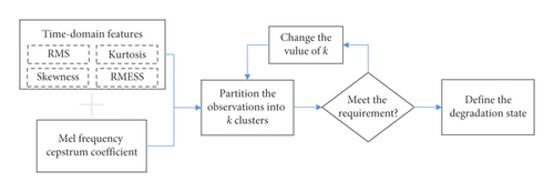
As long as the bearing degradation signal in different time periods can be divided into different categories through these extracted features, the whole degradation process can be divided into different states according to these certain time periods. Figure 1 shows the process of definition of degradation states. Firstly, time-domain features and MFCC features have to be extracted from bearing vibration signals. These features together form input of k-means clustering. Then, change the value of k and observe the distribution of features until all the features can be divided into some continuous time periods, in which features in any time period belong to some specific categories, and at the same time, there is no overlap between the categories of features in different time periods as far as possible. Under these circumstances, degradation states of the bearing can be defined according to the boundary of these certain time periods.

Details are in the caption following the image — **Figure 1**
Open in figure viewer PowerPoint

Typical CNN architecture.

2.2. CNN Recognition Model

Convolutional neural network is a class of deep, feed-forward artificial neural networks. CNNs use a variation of multilayer perceptrons designed to require minimal preprocessing [14]. As shown in Figure 2, a CNN consists of an input layer and an output layer, as well as multiple hidden layers. The hidden layers typically consist of convolutional layers, pooling layers, fully connected layers, and normalization layers.

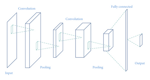
Input in our work is bearing vibration signals, and these signals are going to be convolved by a set of learnable filters, which have a small receptive field, but extend through the full depth of the input volume. Then, max pooling is used to partition the extracted features into a set of nonoverlapping rectangles and, for each such subregion, outputs the maximum [15]. After several convolutional and max pooling layers, all activations are computed by a fully connected layer, and finally, the recognition result is given.

2.3. Architecture of Proposed Model

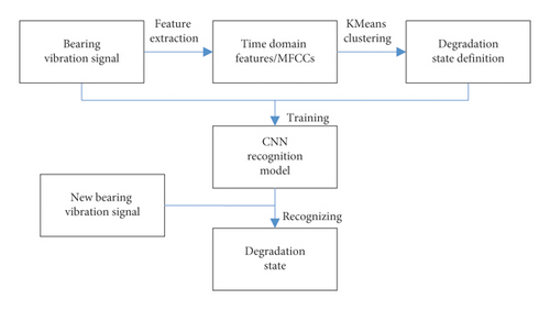
The process of feature extraction is always influenced by human subjectivism, and this will have effect on recognition result. In order to decrease subjective effect, feature extraction is only used to define degradation state of the rolling bearing. It is the original bearing vibration signal that serves as input of the CNN recognition model, and the CNN model is able to learn features by itself by means of its extreme nonlinear fitting capability.

The proposed method has the goal to define and recognize the degradation state of the rolling bearing. Figure 3 shows the architecture of this method, and the role of each procedure is explained as follows.

Step 1. Feature extraction: the time-domain signal processing methods and Mel-frequency cepstral coeffcients feature extraction method are used to extract the features including RMS, kurtosis, skewness, RMSEE, and MFCCs from original bearing vibration signals.
Step 2. Define bearing degradation state by k-means: the aforementioned features together constitute the multidimensional input vector of k-means. Find the certain k value which can let the input vectors be divided into a few categories well by changing the number of clusters and then define the degradation states according to the clustering results.
Step 3. Building and training CNN recognition model: establish the CNN recognition model by setting appropriate network structure. Mark the original bearing degradation signal with the states defined by k-means, and use these labeled data to train the CNN recognition model until it achieves satisfactory results both on training set and test set.
Step 4. Degradation state recognition: now, the well-trained CNN recognition model can be used to recognize degradation state of the rolling bearing.

3. Experiment

In order to verify the feasibility and reliability of the proposed method on degradation state recognition of the rolling bearing, a validation experiment is conducted.

3.1. Dataset Description

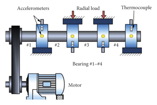
The rolling bearing vibration signals provided by the Center for Intelligent Maintenance System (IMS) are used in this experiment [16]. As shown in Figure 4, four Rexnord ZA-2115 double row bearings are installed on a shaft. The rotation speed is kept constant at 2000 rpm, and a radial load of 6000 lbs is applied onto the shaft and bearing. The experimental dataset is generated from bearing run-to-failure test with the sampling rate as 20 kHz. The run-to-failure test lasts seven days, and finally, outer race failure occurs in bearing 1.

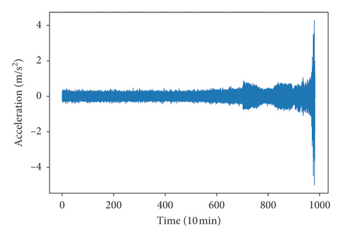
Vibration signals of bearing 1 were used in this paper. Figure 5 shows this rolling bearing’s vibration signal. Obviously, fluctuations become larger at the end of service life, which indicates that bearing failure occurs.

3.2. Degradation States Definition

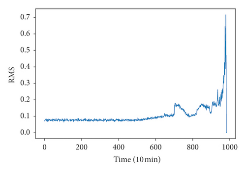
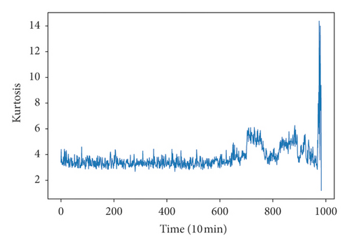
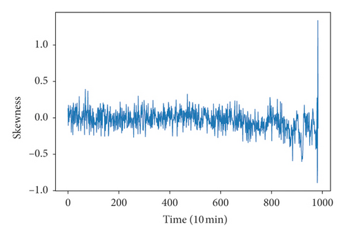
Because run-to-failure signals are unlabeled data, it is necessary to define degradation states so that the CNN recognition model can be trained. K-means clustering of time-domain features and MFCC features were used to define the degradation state. Time-domain features included RMS, kurtosis, skewness, and RMSEE. On extracting the FMCC features, each segment of the signal was further broken into 14 frames of equal duration, and the number of extracted MFCC features is 8. Figure 6 shows the RMS, kurtosis, skewness, RMSEE, and the first two dimensions of MFCCs. It was difficult to define degradation state directly by this figure although there were some obvious fluctuations in the figure; hence, the clustering method was used.

These twelve features formed the input vectors X where each x_i was a 12-dimensional vector. Then, k centroids were set randomly. The category which x_i belonged to could be computed:

\begin{matrix} c_{i} = \arg_{j} \min {‖x_{i} - u_{i}‖}^{2}, \end{matrix}

(9)

where

x_{i} = ({RMS}_{i}, {kurtosis}_{i}, {skewness}_{i}, {RMSEE}_{i}, {MFCC}_{i}^{1}, {MFCC}_{i}^{2}, \dots, {MFCC}_{i}^{8})

, u_j means j^th centroid, and c_i means the ordinal number of the category which x_i belongs to.

Then, new centroids could be computed:

\begin{matrix} u_{j} = \frac{\sum 1 \{c_{i} = j\} x_{i}}{\sum 1 \{c_{i} = j\}} . \end{matrix}

(10)

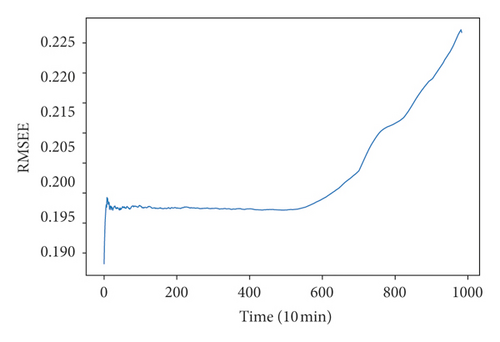
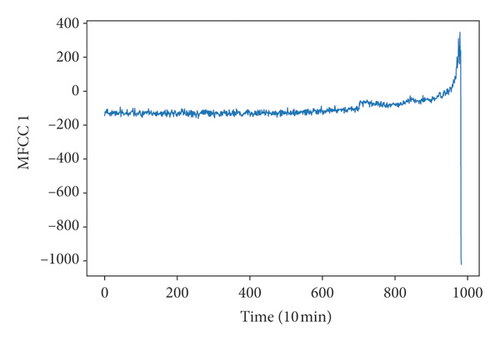
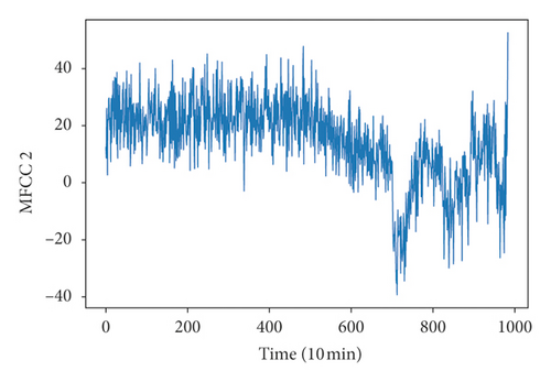
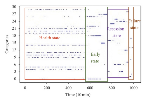
Clustering results could be gotten by repeating these two steps until centroids stop changing. After some trial, we found when k was equal to 30, and the clustering results were easy to distinguish. The clustering results are shown in Figure 7. It could be seen that the features of bearing vibration signals in the whole degradation stage were well divided into some of the 30 categories, and these features as well could be divided into four classes according to the rule that all the features can be divided into some continuous time periods, in which features in any time period belong to some specific categories, and at the same time, there is no overlap between the categories of features in different time periods as far as possible. The first class named health state consisted of the vibration signals in the red rectangle; the second class named early state consisted of the vibration signals in the green rectangle; the third class named recession state consisted of the vibration signals in the violet rectangle; and the fourth class named failure state consisted of the vibration signals in the brown rectangle. So, vibration signals in the first 89 hours were in health state; vibration signals between 90 and 124 hours were in early state; vibration signals between 125 and 158 hours were in recession state; and vibration signals between 158 and 166 hours were in failure state. Although some categories included signals in different states, for example, most signals belonging to category 26 were in early state, but still a few signals were in health state. The reason for this might be noise, and it could be ignored when defining the degradation state. Then, bearing vibration signals could be labeled according to the definition of the degradation state.

3.3. Recognition Model Building

CNN has good ability for recognition. The more the layers of CNN, the stronger the ability to express data. But too many layers are not better because it will increase the training cost and even lead to overfitting. Meanwhile, the selection of parameters of each layer will have influence on network performance [18]. For the sake of a better recognition model, the control variate method [19] was used to determine the network structure and parameters.

Figure 8 shows the degradation recognition model built in this work. “Cov 11s4, 96/ReLU” means a convolution layer with 96 kernels of size 11 with a stride of 4 pixels, and rectified linear unit (ReLU) activation function is used. “Maxpool 3s2” means a max pooling layer of size 3 with a stride of 2 pixels. “FC 4096/ReLU” means a fully connected layer with 4096 neurons, and ReLU activation is used. “Dropout 0.5” means drop 50 percent of input units. “FC 4/Softmax” means a fully connected layer with 4 neurons, and Softmax activation function is used. The number of output layer’s units was 4 because bearing degradation states were divided into 4 classes, which included health state, early state, recession state, and failure state.

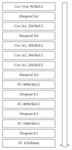
Raw data were collected from the bearing run-to-failure test which lasted seven days, so constructing samples were necessary. In order to ensure the effectiveness of each data sample, the number of data points a sample contained must bigger than the amount of data generated from one turn of a bearing. In this work, a data sample contained 1000 data points, and a 30-second collection interval was used. After sample construction, the data samples were divided into training set and validation set in the proportion eight to two. The training set was used to train the CNN recognition model, and the test set was used to evaluate the classification accuracy of the trained model.

4. Results and Discussion

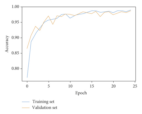
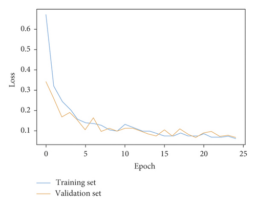
Training set, which took up 80 percent of the data samples, was used to train the CNN recognition model. During the training process, minibatch gradient descent and adaptive moment estimation were used to update the parameters of the model. Twenty percent of the data samples was used to validate the model performance. Figure 9 shows the changes of accuracy rate and loss value during the training process. Obviously, the accuracy rate increased rapidly after starting training and then converged gradually. Correspondingly, the loss value decreased rapidly after starting training and then converged gradually. The accuracy rate on the training set reached 90%, 95%, and 98% after 3, 6, and 15 epochs, respectively. The accuracy rate on the validation set reached 90%, 95%, and 98% after 2, 8, and 14 epochs, respectively. That is to say the CNN recognition model had good generalization performance on the validation set. Finally, the accuracy rate on the training set and validation set reached 98.89% and 98.58% after 25 epochs, respectively.

We tested the model with 3000 new rolling bearing vibration signal samples in order to further verify the feasibility and reliability of the recognition model. As shown in Figure 10, category 0 represented health state; category 1 represented early state; category 2 represented recession state; and category 3 represented failure state. The number in each square represented the number of recognized vibration signal samples. For example, 1667 in the first row and first column meant that 1667 vibration signal samples, which belonged to category 0, were recognized as category 0. These classifications were correct because the actual category was the same as the classification category. Thirty three in the second row and first column meant that there were 33 vibration signal samples, which belonged to category 1, but were misrecognized as category 0.

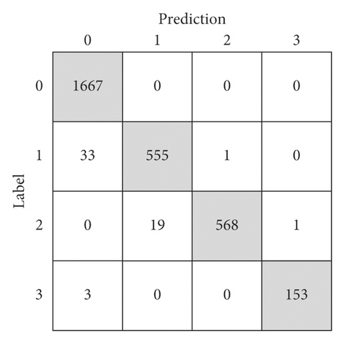
2943 in 3000 rolling bearing vibration signal samples were recognized correctly, so the accuracy on the test set reached 98.10%, which indicated again that the CNN recognition model did well in degradation state recognition of the rolling bearing. Nevertheless, there were 33 vibration signal samples belonging to category 1 but were recognized as category 0, and 19 vibration signal belonging to category 2 but were recognized as category 1. One explanation could be that some vibration signals on the state partition boundary were not able to be recognized easily.

5. Conclusions

(1)
Signal processing methods are used to extract the time-domain features such as RMS, kurtosis, skewness, RMSEE, and Mel-frequency cepstral coefficients feature from original rolling bearing vibration signals. Then, these features together constitute the high-dimensional vectors, which play the role of inputs of the k-means algorithm. Let these vectors be divided into some categories by changing the number of clusters, and finally, the classes of degradation states can be defined effectively according to the clustering results.
(2)
Convolutional neural network has a strong nonlinear fitting ability and is good at extracting features by itself. Taking original bearing vibration signal as input of the CNN recognition model can eliminate interference brought by human factors.
(3)
The proposed architecture of degradation state recognition of the rolling bearing was tested by an experiment. The rolling bearing run-to-failure vibration signals provided by IMS were used. The degradation states were divided into four classes including health state, early state, recession state, and failure state by k-means clustering. Then, the CNN model obtained an excellent recognition performance as the accuracy on training set, validation set and test set are all over 98%. So, the conclusion can be drawn that the proposed method is feasible and reliable to recognize the degradation state of unlabeled rolling bearing signals.

Conflicts of Interest

There are no conflicts of interest regarding the publication of this paper.

Open Research

Data Availability

The data used to support the findings of this study are available from the corresponding author upon request.

References

1 Tao J., Liu Y. L., Fu Z., Yang D. L., and Tang F., Fault damage degrees diagnosis for rolling bearing based on Teager energy operator and deep belief network, Journal of Central South University (Science and Technology). (2017) 48, no. 1, 61–68.
Google Scholar
2 Yuwono M., Qin Y., Zhou J., Guo Y., Celler B. G., and Su S. W., Automatic bearing fault diagnosis using particle swarm clustering and Hidden Markov Model, Engineering Applications of Artificial Intelligence. (2016) 47, 88–100, https://doi.org/10.1016/j.engappai.2015.03.007, 2-s2.0-84948568973.
10.1016/j.engappai.2015.03.007
Web of Science® Google Scholar
3 Kedadouche M., Liu Z., and Thomas M., Bearing Fault feature extraction using autoregressive coefficients, linear discriminant analysis and support vector machine under variable operating conditions, Applied Condition Monitoring. (2018) 9, 339–352, https://doi.org/10.1007/978-3-319-61927-9_32.
10.1007/978-3-319-61927-9_32
Google Scholar
4 Zhang L., Huang W. Y., and Xiong G. L., Assessment of rolling element bearing fault severity using multi-scale entropy, Journal of Vibration and Shock. (2014) 33, no. 9, 185–189.
Google Scholar
5 Ali J. B., Saidi L., Chebel-Morello B., and Fnaiech F., A new enhanced feature extraction strategy for bearing remaining useful life estimation, Proceedings of the International Conference on Sciences & Techniques of Automatic Control & Computer Engineering, December 2015, Monastir, Tunisia, 365–370.
Google Scholar
6 Dong S. J., Yin S. R., Tang B. P., Chen L. L., and Luo T. H., Bearing degradation process prediction based on the support vector machine and markov model, Shock and Vibration. (2014) 2014, 15, 717465, https://doi.org/10.1155/2014/717465, 2-s2.0-84898048626.
10.1155/2014/717465
Web of Science® Google Scholar
7 Soualhi A., Razik H., Clerc G., and Doan D. D., Prognosis of bearing failures using hidden markov models and the adaptive neuro-fuzzy inference system, IEEE Transactions on Industrial Electronics. (2014) 61, no. 6, 2864–2874, https://doi.org/10.1109/tie.2013.2274415, 2-s2.0-84891769069.
10.1109/TIE.2013.2274415
Web of Science® Google Scholar
8 Chen J. X., Cheng L. S., Yu H., and Hu S. L., Health status assessment for complex systems based on EMD-SVD and Mahalanobis-Taguchi system, Systems Engineering and Electronics. (2017) 39, no. 7, 1542–1548.
Google Scholar
9 Ali J. B., Chebel-Morello B., and Saidi L., Accurate bearing remaining useful life prediction based on Weibull distribution and artificial neural network, Mechanical Systems & Signal Processing. (2015) 56-57, 150–172, https://doi.org/10.1016/j.ymssp.2014.10.014, 2-s2.0-84919729802.
10.1016/j.ymssp.2014.10.014
Web of Science® Google Scholar
10 Napoleon D. and Pavalakodi S., A new method for dimensionality reduction using KMeans clustering algorithm for high dimensional data set, International Journal of Computer Applications. (2011) 13, no. 7, 41–46, https://doi.org/10.5120/1789-2471.
10.5120/1789-2471
Google Scholar
11 Hossan M. A., Memon S., and Gregory M. A., A novel approach for MFCC feature extraction, Proceedings of the International Conference on Signal Processing and Communication Systems, December 2010, Gold Coast, Australia, 1–5.
Google Scholar
12 Nelwamondo F. V. and Marwala T., Faults detection using Gaussian mixture models, mel-frequency coefficients and kurtosis, Proceedings of the 2006 IEEE International Conference on Systems, Man and Cybernetics, October 2006, Taipei, Taiwan, 290–295.
Google Scholar
13 Wang Z., Willett P., DeAguiar P. R., and Webster J., Neural network detection of grinding burn from acoustic emission, International Journal of Machine Tools and Manufacture. (2001) 41, no. 2, 283–309, https://doi.org/10.1016/s0890-6955(00)00057-2, 2-s2.0-0035149341.
10.1016/S0890-6955(00)00057-2
Web of Science® Google Scholar
14 Lecun Y., Bottou L., Bengio Y., and Haffner P., Gradient-based learning applied to document recognition, Proceedings of the IEEE. (1998) 86, no. 11, 2278–2324, https://doi.org/10.1109/5.726791, 2-s2.0-0032203257.
10.1109/5.726791
Web of Science® Google Scholar
15 Tolias G., Sicre R., and Jégou H., Particular object retrieval with integral max-pooling of CNN activations, 2015, Computer Science, https://arxiv.org/abs/1511.05879.
Google Scholar
16 Qiu H., Lee J., Lin J., and Yu G., Wavelet filter-based weak signature detection method and its application on rolling element bearing prognostics, Journal of Sound and Vibration. (2006) 289, no. 4-5, 1066–1090, https://doi.org/10.1016/j.jsv.2005.03.007, 2-s2.0-33644547646.
10.1016/j.jsv.2005.03.007
Web of Science® Google Scholar
17 William G., Jérôme A., and François G., Analysis of the rolling element bearing data set of the center for intelligent maintenance systems of the university of cincinna, Proceedings of the 13th International Conference on Condition Monitoring and Machinery Failure Prevention Technologies, October 2016, Paris, France.
Google Scholar
18 Hinton G. E., A practical guide to training restricted Boltzmann machines, Lecture Notes in Computer Science, 2012, 9, no. 1, Springer Nature, Basingstoke, UK, 599–619, https://doi.org/10.1007/978-3-642-35289-8_32.
Google Scholar
19 Grathwohl W., Choi D., Wu T., Roeder G., and Duvenaud D., Backpropagation through the Void: optimizing control variates for black-box gradient estimation, Proceedings of the International Conference on Learning Representations, May 2018, Vancouver, Canada.
Google Scholar

Citing Literature

All articles

Degradation State Recognition of Rolling Bearing Based on K-Means and CNN Algorithm

Abstract

1. Introduction

2. Methods of Bearing Degradation State Recognition