Vibration Reliability Evaluation of Main Fan Spindle Bearings
Abstract
Based on an analysis of failure causes, the axial force is the main reason why spindle bearings vibrate abnormally and cause frequent failures of the main fans in mines. In this paper, the probability density function of the spindle bearing vibration was established through the bootstrap maximum entropy method, the Lagrangian multiplier and the empirical coefficient were introduced, and models of the upper- and lower-bound functions of the probability density and the true value function of the failure probability were established. The true value function and interval estimation values of vibration reliability were obtained on the basis of maximum entropy. The analysis results showed that the estimation true values of vibration decreased with an increase in the empirical coefficient. When the empirical coefficient was less than 0.1, the estimated true value decreased sharply. When the empirical coefficient was greater than 0.1, the vibration value decreased linearly with the empirical coefficient. When the empirical coefficient was 0.1, the estimated true value was 0.85 mm/s2, which is consistent with the change in the actual vibration value. Therefore, when the main fan is fault predicted, the vibration value should be 0.85 mm/s2 as the basis for judgment and then the theoretical basis for the fault diagnosis of the spindle bearing are provided.
1. Introduction
As one of the fixed equipment in a coal mine, the main fan is responsible for conveying enough fresh air into the coal mine. This fresh air dilutes and discharges harmful gases and dust such as gas and carbon monoxide and ensures the safe operation of the coal mine. The performance and operating conditions of the main fan directly determine the safety of mine workers and the production efficiency in the coal mine [1–3]. The performance of the main fan, in turn, depends largely on the performance of its spindle bearings. During the actual operation, the main fan is subjected to additional impact loads owing to changes in ventilation and nonuniform deformation caused by installing the fan. All these loads are transferred to the bearings, thereby straining their working conditions and eventually causing them to fail. As a result, the fan would shut down and lead to major safety hazards. According to survey data, the failure of bearings accounts for more than half of the fan failures directly or indirectly. For example, fractures in the bearings of the main fan in the Qinling Power Plant, located in Shanxi Province of China, caused the fan to malfunction and resulted in grave accidents [4]. Therefore, in this paper, a reliability evaluation method for the spindle bearing is proposed, which provides a theoretical basis for the early fault warning processing of the bearing and is one of the necessary means to avoid malfunctioning of the main fan.
Due to high test cost, the spindle bearings of the main fan in the coal mine lack enough test data, and so the prior information of the bearings is uncertain. There are many difficulties to evaluate the reliability of the bearings. These include the operating conditions that surround these bearings and lack enough test data. The cost of the bearing itself and that of its testing are also considerations. Xia et al. [5, 6] proposed a bearing evaluation model without prior information to solve the problem of evaluation of zero-failure data with unknown probability. Liu et al. [7] developed a prediction model of ammunition storage reliability in the natural storage state where the main affecting factors of ammunition reliability include temperature, humidity, and storage period. A new improved algorithm based on three-stage ant colony optimization (IACO) and BP neural network algorithm is proposed to predict ammunition failure numbers. Research results showed that the IACO-BP algorithm has better accuracy and stability in ammunition storage reliability prediction than the BP network, PSO-BP network, and ACO-BP algorithm. Li et al. [8] used the Bayes method to introduce failure data into the confidence interval and established the modified one-sided confidence evaluation method. The validity of the method was verified by experiments. Zhao et al. [9] used the failure factor and the adaptive coefficient to introduce the failure data and proposed an improved integrated E-Bayesian method to evaluate the avionics equipment, which proved that the method has better evaluation performance. On the basis of extracting the characteristics of the time domain, frequency domain, and time-frequency domain of the bearings, Wang et al. [10] proposed the improved logistic regression model with the principal component analysis method and obtained the bearing reliability curve and verified the correctness of their method. Preeti and Manisha [11] dealt with the design of the optimal ramp-soak-stress accelerated degradation test using the Wiener process for modeling degradation paths. The accelerated degradation test is incorporated in the zero-failure reliability demonstration test to facilitate reduction in the test duration resulting in reduction in the test cost of high-reliability items. Kwon [12, 13] used the Bayes theory to predict the reliability of products obeying the Weibull distribution and the lognormal distribution. Yang et al. [14] proposed a new Bayesian method based on engineering knowledge and mathematical relation to obtain more accurate results of the reliability assessment for a small sample size (less than 12) and zero-failure data. Kan et al. [15] established the zero-failure data form and the corresponding Bayesian model to solve the zero-failure problem of the numerical control machine tools, and an expert-judgment process that incorporates prior information was presented to solve the difficulty in obtaining reliable prior distributions of Weibull parameters. Furthermore, the proposed reliability model and assessment method under the zero failure of NCMTs was validated. Yin et al. [16] proposed a reliability analysis method based on the E-Bayesian estimation for zero-failure data. The precision of estimation results of reliability increased significantly based on the hierarchical Bayesian estimation. Li et al. [17] built a Bayes model of the zero-failure problem for a single NC machine tool and presented the method of building the prior distributions of Weibull parameters. The method can be said to be a standard solution to the zero-failure reliability assessment for NC machine tools. Jiang et al. [18] presented a method to estimate the intervals of the failure probability for the Weibull distribution by using the concavity and the property of the distribution function and validated the effectiveness and robustness of the method. Xu and Zhixin [19] proposed a fuzzy Bayesian-based zero-failure accelerated degradation demonstration (ADD) test method. This method takes the three uncertainties into account and is optimized based on the target of minimizing the test cost with a minimum sample size. Li et al. [20] presented a method to study the point estimates of reliability and confidence interval estimates of reliability. Wang et al. [21] built the novel method based on the kernel principal component analysis (KPCA) and the Weibull proportional hazards model (WPHM) to assess the reliability of rolling bearings. A high relative feature set was constructed by selecting the effective features through extracting the time domain, frequency domain, and time-frequency domain features over the bearing’s life cycle data. Li et al. [22] proposed a new reliability assessment method based on the hidden Markov model considering performance degradation, called degradation-hidden Markov model for wind turbines, as expensive large-scale equipment with long lifetime face with the dilemma of lacking enough statistical data and leads to insufficiency reliability data for field operations.
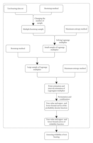
This discussion shows that many researchers have carried out research on products with unknown probability and known probability and have obtained many beneficial results. However, owing to their special operating conditions, not only the prior information but also the test data are scarce for the spindle bearings of the main fan. Only a certain amount of zero-failure test data can be collected during the actual operation of the main fan. However, owing to significant variations in the working conditions of different coal mines, the operating conditions for bearings also vary widely. In view of this, based on the vibration data of the spindle bearings in the actual operation process, the bootstrap resample method is adopted to deal with the meager sample information on the bearings. Compared with other methods, the method can be used to study the data, which is the small sample of the zero-failure, and the probability distribution of the data is unknown. The method abandons the Lagrangian multiplier as a constant and establishes the probability density function of bearing vibration based on a large amount of data obtained by the bootstrap method. By changing the number of samples, different Lagrangian multipliers and the parameter estimation interval are obtained based on the maximum entropy method. Then, the upper and lower limits of the Lagrange multiplier are obtained, and different multiple probability density functions and reliability functions are acquired. Finally, the interval estimation of the reliability function is obtained according to the principle of minimum uncertainty. The spindle bearing of the coal mine fan is evaluated for reliability so as to provide a theoretical basis for their fault diagnosis.
2. Mathematical Model
Based on the bootstrap principle, the reliability evaluation model of spindle bearings of the main fan is established by using resampling and the maximum entropy method.
2.1. Bootstrap Principle
2.2. Probability Density Function
The maximum entropy method is used to estimate the acquired vibration value optimally. Furthermore, the Lagrange multiplier is used to solve the extreme value of the objective function.
It is difficult to solve the probability distribution through the maximum entropy method. In this paper, the Newton iteration method of interval mapping is proposed to solve the probability distribution. The selection of the integral mapping interval is the key to the solving process. Furthermore, the original data are processed by using the histogram method. The original zero-failure data are arranged in an increasing order and divided into groups of j to draw the histogram (histogram width ΔX = (Xmax − Xmin)/n); the value of the group (the midpoint value of each square width), namely, ξq, and pq (the number of data falling in each of the square widths or the ratio of the number of data falling in each of the square widths to the total number of original data) can be obtained as q = 2,3, …, j + 1. Then, the histogram is expanded to the j + 2 group, and it is assumed that p1 = pj+2 = 0.
To facilitate convergence, the raw data sequence is nondimensionally mapped onto interval [−e, e] [5].
2.3. Upper and Lower Limits of the Probability Density Function
2.3.1. Interval Estimation of Lagrangian Multiplier
According to the aforementioned analysis, the Lagrangian multiplier is taken as a variable and the bootstrap resampling method is used to estimate the interval of the Lagrange multiplier based on the maximum entropy principle.
2.3.2. Point Estimate of Mapping Parameters
2.3.3. Solving the Upper- and Lower-Bound Functions of the Probability Density Function
From the principle of minimum uncertainty, the two curves closest to the curve of the true value function can be found, and the two curves are the upper- and lower-limit functions of the maximum entropy probability density fU(x) and fL(x).
2.4. Interval Estimation of the Reliability Function
A flowchart of the proposed method is shown in Figure 1.
3. Bearing Vibration Reliability Assessment
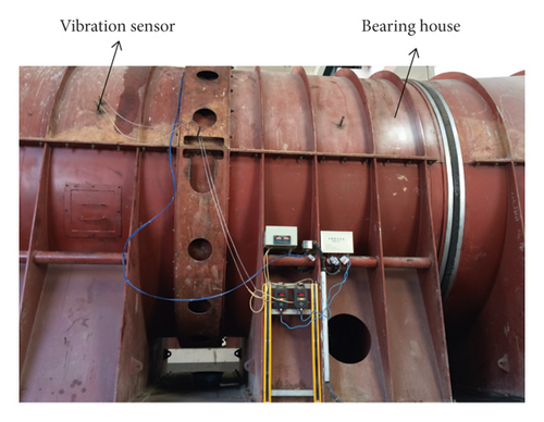
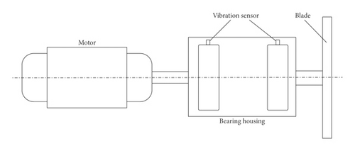
The coal mine enterprise in Shanxi Province uses the NMAF3750/2135-1B main fan. The main fan parameters are given in Table 1. The experimental data sets were generated from bearing under actual conditions, as shown in Figure 2.
| Motor model | YVVF800-8 |
|---|---|
| Motor power | 4000 kW |
| Rated flow | 650 m3/s |
| Full pressure | 6500 Pa |
| Rated speed | 740 r/min |
| Wheel and blade quality | 60000 kg |
| Diameter of air duct | 3750 mm |
| Single-row angular contact ball bearing | FAG 7244-B-MP-UA |
| Single-row cylindrical roller bearing | FAG NU344-E-M1 |
| Bearing lubricant | 46 Turbine oil |
- (1)
Abnormal vibration occurs in the bearing housing, and the vibration acceleration increases gradually with time, increasing until the bearings are damaged. This phase lasts approximately one month.
- (2)
After the main fan is running for a period of time, abnormal noise occurs in the bearing housing.
- (3)
Axial scratches appear on the rolling elements of cylindrical roller bearings, and the scratches become very obvious. The first damaged bearings show significant scratches on multiple rolling elements. Axial scratches also appear on the second damaged bearing rolling element. The scratches are approximately symmetrically distributed, as shown in Figure 3.
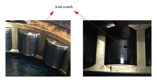
After analyzing the main shaft structure of the main fan and its installation method, the analysis of the spindle force, the spindle bearings are subjected to a large axial force, while the cylindrical roller bearing located on the side of the fan cannot withstand large axial loads, so it is easy to cause roller scratches. On-site spindle bearing vibration monitoring shows that the bearing vibration value increases very fast. After one month, the bearing vibration value exceeds the limit value, and the bearing is damaged. From the bearing vibration test and the vibration value record tables, a set of zero-failure data with significant changes in the bearing vibration value is extracted, as shown in Figure 4. The bearings are evaluated for reliability using the measured zero-failure data.

Using the bootstrap resampling method, 15 data sets are extracted each time a total of 30,000 times. The obtained data are shown in Figure 5.
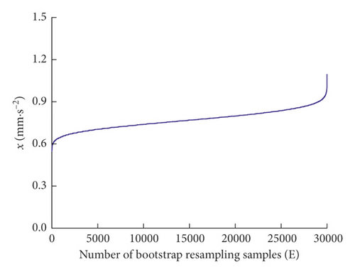
Changing the number of samples l, extraction 30,000 times, the Lagrangian multiplier and mapping parameters are shown in Tables 2 and 3.
| l | λ 0 (t) | λ 1 (t) | λ 2 (t) | λ 3 (t) | λ 4 (t) | λ 5 (t) |
|---|---|---|---|---|---|---|
| 4 | 0.764017 | −0.893 | −0.676775 | −0.0572752 | −0.0438363 | 0.0179277 |
| 5 | 0.995605 | −0.640203 | −0.658176 | −0.0122686 | −0.0532785 | 0.013914 |
| 6 | 1.1555 | −0.60576 | −0.74638 | 0.041612 | −0.044281 | 0.0087823 |
| 7 | 1.2018 | −0.699 | −0.8527 | 0.039447 | −0.034817 | 0.0043786 |
| 8 | 1.3268 | −0.5377 | −0.88499 | 0.016575 | −0.04083 | 0.010802 |
| 9 | 1.306 | −0.80632 | −0.98232 | 0.038709 | −0.019284 | 0.005684 |
| 10 | 1.4717 | −0.3734 | −0.93702 | −0.035129 | −0.02088 | 0.020692 |
| 11 | 1.4927 | −0.51352 | −0.9219 | 0.067689 | −0.024538 | 0.00033619 |
| 12 | 1.4463 | −0.86541 | −1.0762 | 0.027183 | −0.0311 | 0.011318 |
| 13 | 1.6262 | −0.33021 | −1.013 | 0.073191 | −0.03635 | −0.0012287 |
| 14 | 1.5302 | −0.85746 | −1.1591 | 0.016319 | −0.032157 | 0.0069138 |
| 15 | 1.5946 | −0.75926 | −1.0768 | 0.021642 | −0.010826 | 0.0031976 |
| l | a(t) | b(t) |
|---|---|---|
| 4 | 5.60792 | −4.85786 |
| 5 | 6.16235 | −5.09626 |
| 6 | 6.68768 | −5.43364 |
| 7 | 6.8496 | −5.5875 |
| 8 | 7.2757 | −5.8478 |
| 9 | 7.4007 | −6.0399 |
| 10 | 8.1008 | −6.4159 |
| 11 | 8.4104 | −6.6746 |
| 12 | 8.1771 | −6.644 |
| 13 | 8.8595 | −6.9375 |
| 14 | 8.5624 | −6.9234 |
| 15 | 9.3847 | −7.5454 |
Assuming the confidence level p = 95% (i.e., α = 0.05), the empirical coefficient ρ = 0.1, and using the obtained 12 λ0 values as bootstrap resample for the new sample, the lower-limit values of the confidence interval are λ0L = 1.20283 and λ0U = 1.46116, respectively. Therefore, the estimated interval of parameter λ0 is [λ0L, λ0U] = [1.20283, 1.46116], of parameter λ1 is [λ1L, λ1U] = [−0.745216, −0.533746], of parameter λ2 is [λ2L, λ2U] = [−1.00388, −0.831147], of parameter λ3 is [λ3L, λ3U] = [0.00207399, 0.04265], of parameter λ4 is [λ4L, λ4U] = [0.00478754, 0.0121292]; and that of parameter λ5 is [λ5L, λ5U] = [−0.0216008, 0.00959115].
The point estimates of parameters a and b available from equation (27) are .
Substituting the Lagrange multiplier upper and lower limits and point estimates of the mapping parameters into equation (28), 64 probability density functions curves are obtained.
By the principle of minimum uncertainty, λ0 = λ0L = 1.20283, λ1 = λ1U = −0.533746, λ2 = λ2U = −0.831147, λ3 = λ3L = 0.00207399, λ4 = λ4L = 0.00478754, and λ5 = λ5L = −0.0216008, the lower-limit curve RL (x) of the reliability function is obtained; λ0 = λ0L = 1.2028, λ1 = λ1U = −0.533746, λ2 = λ2L = −1.00388, λ3 = λ3U = 0.04265, λ4 = λ4L = 0.00478754, and λ5 = λ5U = 0.00959115, the upper-limit curve RU(x) of the reliability function is obtained. The reliability upper and lower bound functions are shown in Figure 6.
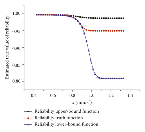
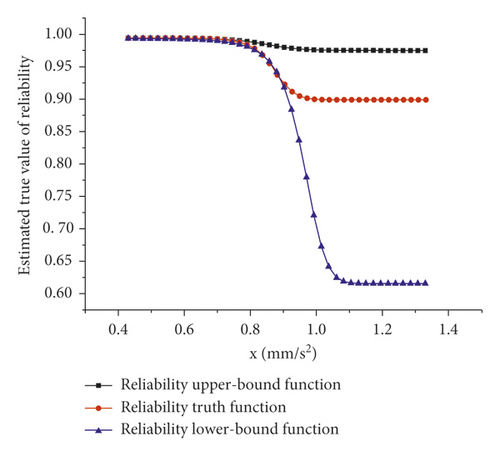
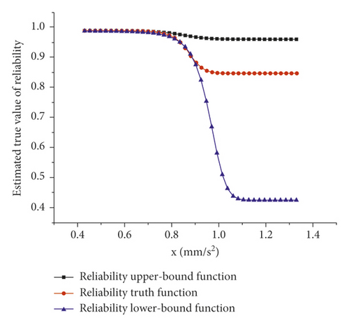
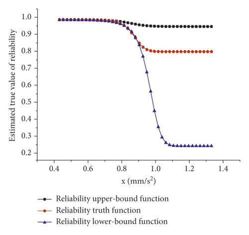
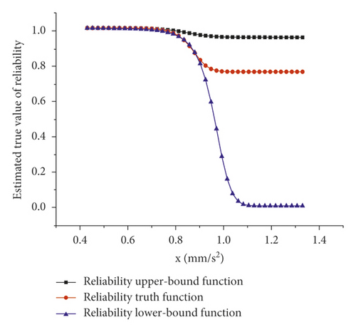
It can be seen from Tables 2 and 3 that when the number of samples is 15, the Lagrangian multipliers λ00, λ10, λ20, λ30, λ40, and λ50 are equal to 1.5946, −0.75926, −1.0768, 0.021642, −0.010826, and 0.003197, respectively, and the mapping parameters are a0 = 9.3847 and b0 = −7.5454. Substituting these parameters into equation (29), the estimated truth function of the probability density function f0(x) can be obtained. f0(x) can be substituted into equations (30)–(32) to obtain the reliability estimate truth value function, as shown in Figure 6.
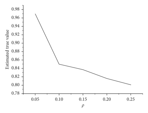
For the same confidence level p = 95% (i.e., α = 0.05), when the empirical coefficients are different, the estimated true value and estimation interval are obtained, as shown in Table 4. The reliability upper- and lower-limit functions and the truth value function are shown in Figure 6.
| Empirical coefficients ρ | 0.05 | 0.1 | 0.15 | 0.2 | 0.25 |
|---|---|---|---|---|---|
| Estimated true value | 0.97 | 0.85 | 0.837 | 0.816 | 0.801 |
| Estimation interval | [0.9000, 0.9875] | [0.9431, 0.9848] | [0.9523, 0.977] | [0.9506, 0.973] | [0.9469, 0.9692] |
| Estimated interval difference | 0.0875 | 0.0417 | 0.0247 | 0.0224 | 0.0151 |
It can be seen from Table 4 and Figures 6 and 7 that the estimated true value decreases as the value of the empirical coefficient increases. Moreover, the estimated interval difference decreases. This indicates that the estimated value is more accurate. It can be seen from Figure 6 that as the empirical coefficient increases, the minimum value of the estimated lower-limit function decreases. When ρ = 0.3, the estimated lower-bound function value is less than 0 (i.e., −0.1507), and the lower-bound function estimate is already inaccurate; therefore, the empirical coefficient must not be greater than 0.3.
In Figure 7, the ordinate is the reliability estimation true value, and the abscissa is the vibration value.
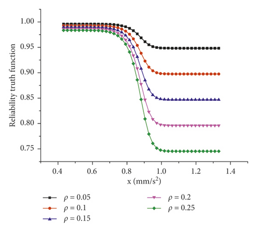
It can be seen from Figure 8 that as the empirical coefficient increases, the estimated value sharply decreases when ρ is less than 0.1 and the estimated true value and ρ decrease substantially linearly when ρ is greater than 0.1. Therefore, the empirical coefficient is a critical value at 0.1. It can be seen from Figure 4 that when the vibration value is greater than 0.84 mm/s2, the vibration value increases substantially linearly; therefore, the empirical coefficient ρ = 0.1 is taken.
It can be seen from Figure 6(b) that the reliability function gradually decreases as the vibration value increases when ρ = 0.1. Before the vibration value reaches 0.75 mm/s2, the upper and lower limits of the reliability function are coincident with the reliability estimation truth function curve, thereby indicating that the reliability estimation function is more accurate. As the vibration value increases, the upper and lower limits of the reliability function deviate further from the estimated truth function curve. When the vibration value is greater than 0.8 mm/s2, the reliability estimation true value and the lower-limit function decrease sharply. This is because the estimation of the reliability function becomes more difficult as the vibration value increases and the dispersion of the vibration value increases. When the confidence level is equal to 0.95, the estimated true value is 0.85 mm/s2. Combined with the above analysis, when the fault of the spindle bearings of the main fan is judged, the vibration value of 0.85 mm/s2 is one of the parameters, and the correctness of the method is also proved.
4. Conclusions
- (1)
The maximum entropy method of grey bootstrap is proposed to establish the vibration probability density function of the spindle bearing. An empirical coefficient is introduced to establish the true value function of the bearing reliability estimation.
- (2)
The bearing reliability estimation true value decreases as the empirical coefficient increases. Moreover, the estimated interval difference also decreases. When the empirical coefficient is equal to 0.1, the estimated true value is more in line with the real situation.
- (3)
When the empirical coefficient is equal to 0.1, the true value of the vibration estimation is equal to 0.85 mm/s2. The vibration value should be one of the bases for the bearing failure warning. This is also the actual working condition—when the actual vibration value of the bearing is greater than 0.84 mm/s2, the bearing vibration increases linearly. Finally, the validity and correctness of the method are verified.
Conflicts of Interest
The authors declare that they have no conflicts of interest.
Acknowledgments
The research was supported by the National Natural Science Foundation of China (Grant nos. 51275155 and 51805151). Pang gratefully acknowledged the helpful discussions with the research group and colleagues in the School of Mechanical and Electrical Engineering at Henan University of Science and Technology.
Open Research
Data Availability
The vibration value data used to support the findings of this study are included within the article.


