Volume 2019, Issue 1 2898219

Research Article

Open Access

Automatic Evaluation of Internal Combustion Engine Noise Based on an Auditory Model

Kai Liang,

Corresponding Author

Kai Liang

[email protected]

orcid.org/0000-0003-4571-187X

Information Technology Center, Luoyang Institute of Science & Technology, Luoyang 471023, China lit.edu.cn

Search for more papers by this author

Haijun Zhao,

Haijun Zhao

School of Automotive and Transportation, Tianjin University of Technology and Education, Tianjin 300222, China tute.edu.cn

National Joint Engineering Research Center of Intelligent Vehicle Infrastructure Cooperation and Safety Technology, Tianjin University of Technology and Education, Tianjin 300222, China tute.edu.cn

Search for more papers by this author

Kai Liang,

Corresponding Author

Kai Liang

[email protected]

orcid.org/0000-0003-4571-187X

Information Technology Center, Luoyang Institute of Science & Technology, Luoyang 471023, China lit.edu.cn

Search for more papers by this author

Haijun Zhao,

Haijun Zhao

School of Automotive and Transportation, Tianjin University of Technology and Education, Tianjin 300222, China tute.edu.cn

National Joint Engineering Research Center of Intelligent Vehicle Infrastructure Cooperation and Safety Technology, Tianjin University of Technology and Education, Tianjin 300222, China tute.edu.cn

Search for more papers by this author

First published: 2019

https://doi.org/10.1155/2019/2898219

Citations: 3

Academic Editor: Radoslaw Zimroz

Share a link

Email
Wechat
Bluesky

Abstract

To improve the accuracy and efficiency of the objective evaluation of noise quality from internal combustion engines, an automatic noise quality classification model was constructed by introducing an auditory model-based acoustic spectrum analysis method and a convolutional neural network (CNN) model. A band-pass filter was also designed in the model to automatically extract the features of the noise samples, which were later used as input data. The adaptive moment estimation (Adam) algorithm was used to optimize the weights of each layer in the network, and the model was used to evaluate sound quality. To evaluate the predictive performance of the CNN model based on the auditory input, a back propagation (BP) sound quality evaluation model based on psychoacoustic parameters was constructed and used as a control. When processing the label values of the samples, the correlation between the psychoacoustic parameters of the objective evaluation and evaluation scores was analyzed. Four psychoacoustic parameters with the greatest correlation with subjective evaluation results were selected as the input values of the BP model. The results showed that the sound quality evaluation model based on the CNN could predict the sound quality of internal combustion engines more accurately, and the input evaluation score based on the auditory spectrum in the CNN classification model was more accurate than the short-time average energy input evaluation score based on the time domain.

1. Introduction

The loudness and sound quality of internal combustion engines directly affect the operator’s experience. Therefore, noise control and evaluation of internal combustion engines is a popular topic in the field of engineering. The objective evaluation methods of noise quality include linear and nonlinear evaluation and predictive models. In previous studies [1, 2], multiple linear regression theory was used to establish a sound quality classification model, the results of which agreed closely with the measured values of subjective evaluation. Huang et al. [3] proposed the use of psychoacoustic parameters as inputs to a genetic algorithm (GA)-wavelet neural network and back propagation (BP) neural network to predict sound quality, which was proven to be somewhat effective. In a study by Xu et al. [2], a nonlinear evaluation model based on an adaptive boosting (AdaBoost) algorithm was proposed. The predictive results of the model were compared with those of the GA-BP, GA-extreme learning machine (ELM), and GA-support vector machine (SVM) models, which showed that the proposed model improved the accuracy and precision. In the above models, the sound qualities were predicted using the objective psychoacoustic parameters of sound quality as inputs. The accuracy and precision of the predictions were the main focus of the evaluation model research. Auditory models are widely used in target recognition, fault diagnosis, and speech recognition. An underwater target echo recognition method based on auditory spectrum features was proposed [4]. The underwater target single-frequency echo recognition experiment showed better robustness. Under the same test conditions, the recognition rate was about 3% higher than that of a perceptual linear prediction (PLP) model. In a study by Wu et al. [5], the auditory spectrum feature extraction was applied to the fault diagnosis of broken teeth. A gammatone (GT) band-pass filter and phase adjustment were applied to signals to calculate the probability density of the amplitude at each extreme point. The results showed that the proposed method could accurately characterize and extract the fault features of broken teeth, and the extraction accuracy was high. Liang [6] proposed a binaural auditory model and applied it to the analysis and control of a car’s interior noise quality. The results showed that the interior noise quality of the car was greatly improved. At present, there have been no studies on the application of auditory models in the automatic evaluation of noise quality of internal combustion engines.

In this study, the noise samples of certain types of diesel engines were processed using a gammatone filter to establish an auditory model similar to human ears, and an automatic classification model of noise quality was constructed based on a convolutional neural network (CNN). We aimed to study the following: (1) time domain signal processing of noise samples, (2) auditory spectrum transformation of noise samples, and (3) applications of the auditory spectrum-based CNN in the classification of noise quality. The auditory model of sound samples was taken as the input, and the subjective evaluation score was taken as the output label for model training and optimization. Compared to the model using objective sound quality psychoacoustic parameters as the input, the proposed model exhibited higher classification accuracy.

2. Auditory Model

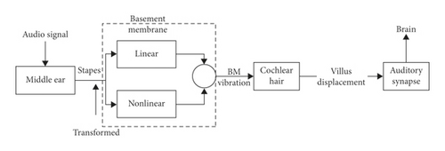
The human auditory system consists of several parts of the ear and brain. The widely used auditory model in the field of signal analysis simulates the ear functions. Different locations of the basement membrane inside the cochlea will produce different traveling wave deflections when stimulated by corresponding frequencies, similar to a set of band-pass filter banks, and the nerve fibers for transmission are called channels. Each channel corresponds to a specific point on the basement membrane. In the human auditory system, each channel has an optimal frequency (center frequency), which defines the frequency of maximum excitation [7], as shown in Figure 1.

Details are in the caption following the image — **Figure 1**
Open in figure viewer PowerPoint

Structure of human auditory model.

Gammatone (GT) band-pass filter [8] banks have been used to simulate the internal mechanism of the cochlea. The frequency channel of the GT filter banks covers the range of 80 Hz–8 kHz. Figure 2 shows the frequency response of the GT filter banks. The GT filter algorithm is represented as follows:

\begin{matrix} y (t, s) = x (t) *_{t} h (t, s), \\ h (t, s) = c t^{(n - 1)} e^{- 2 π b t} \cos (2 π f_{s} t + φ) u (t) . \end{matrix}

(1)

The sound sample x was decomposed into 64 different frequency channels using GT filter banks. Each frequency channel contained the relationship between the component harmonics and time t. y(t, s) denotes the auditory spectrum output of basement membrane, x(t) denotes sample signal, ∗_t denotes time domain convolution, h(t, s) denotes the time domain expression of the GT filters, f_s denotes central frequency coverage, which was set to 50 Hz–20 kHz, u(t) denotes step function, and n denotes the order number of the filters. Studies have shown that when n = 4, the characteristics of the human ear basement membrane filter can be well simulated using GT filters. The phase φ is 0, and b denotes the equivalent rectangle bandwidth (ERB), i.e., the attenuation velocity of the filter, calculated as follows:

\begin{matrix} b = b_{1} * ERB (f), \\ ERB (f) = 24.7 * (0.004371.0 f +) . \end{matrix}

(2)

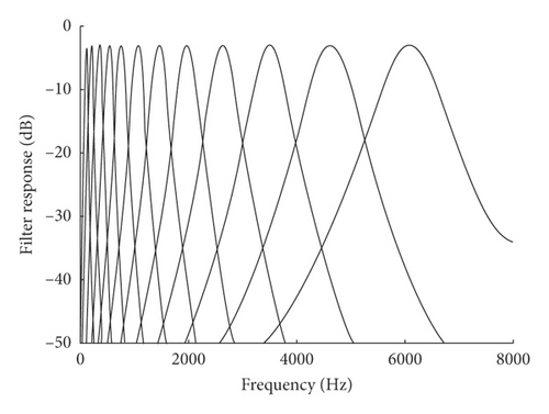
The value of b₁ was 1.019, so that the physiological parameters of basement membrane could be better simulated.

3. Automatic Evaluation Method

The idea of an unsupervised learning algorithm in machine learning was adopted for automatic evaluation. A CNN model was chosen to automatically extract the eigenvalues of the input noise samples, and the parameters that were learned through training were applied to the online automatic evaluation system to continuously optimize the model and improve the classification accuracy.

3.1. Evaluation Based on CNN

A CNN [9] is a deep feed-forward artificial neural network to which a convolution layer and pooling layer are added. It can be used to extract the features of training samples under unsupervised conditions, realize sparse representation of sample features, and achieve the principle of detecting optical signals similar to animal visual cortex neurons.

The use of CNNs has been highly successful in the field of image and speech recognition. The convolution layer of a CNN involves sparse interactions and parameter sharing, so that each convolution kernel can extract the feature information on the time-frequency axis of the sample sound, which is directly related to the sound quality perception.

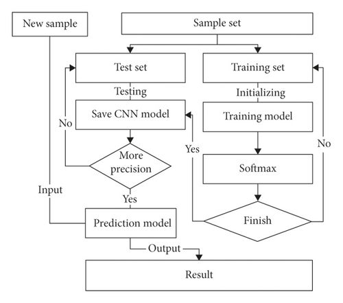
The preprocessed sound samples and subjective evaluation results were divided into two parts: a training set and a test set. The training set data were taken as the original input to train the CNN model. A Softmax classifier was used to obtain the attribution probability of the current samples. The test set was used to validate the training model completed iteratively, and the optimal model was selected and saved. Thus, the saved CNN classification model could be used to predict the attributes of new samples. The process is shown in Figure 3.

3.2. Definition of CNN Evaluation Model

The input layer data sample V ∈ R^A×B. A denotes the number of frames contained in a noise sample. B denotes the dimension of each frame (it was set to 64), as audio frames were signals obtained through the gammatone band-pass filter, and the dimension ordinal number indicates that the frequencies of the feature points in this frame were arranged in ascending order. The vertical coordinates of the input data in the figure are frequency bands. v^l−1 denotes eigenvalue v^l−1 = [v₁, v₂, …, v_b] of the l − 1^th layer, and v_b denotes the eigenvalue of the b^th band. The convolution kernel of the l layer

k^{l} = [k_{1}^{l}, k_{2}^{l}, k_{3}^{l}, k_{4}^{l}]

. It consists of four convolution kernels, and the activation value

v_{j}^{l}

of the convolution layer was calculated as follows:

\begin{matrix} v_{j}^{l} = f (\sum_{i \in A}^{s} v_{i}^{l - 1} * k_{j}^{l} + b_{j}) . \end{matrix}

(3)

The left side denotes the j^th feather map of layer l. A convolution calculation was performed on all feature maps

v_{i}^{l - 1}

of layer l − 1 and the j^th convolution kernel

k_{j}^{l}

of layer l. The right side was obtained by adding the sum and the offset b_j of the j^th feature map. Further, it was calculated using an activation function f(x), which was a rectified linear unit (ReLU) function [10], shown as follows:

\begin{matrix} f (x) = \max (0, x) . \end{matrix}

(4)

The pooling layer [11] was the next operation for the convolution layer. The low-resolution representation of the feature map obtained by the convolution layer was calculated using a downsampling method. A maxpooling function is often used to calculate the maximum value of a feature map obtained by convolution (continuous frequency band), and its formula is as follows:

\begin{matrix} p_{j, m} = Max (v_{j, (m - 1) \times n + k}), k = 1, \dots, r, \end{matrix}

(5)

where p_j,m denotes the output of the j^th feature map of the m^th pooling band, n denotes the downsampling factor, and r denotes the size of pool, indicating how many frequency bands of data were pooled together. The parameter sharing and maxpooling of convolution kernels in the model played an important role in the invariance of small frequency shift characteristics and could reduce the number of training parameters to suppress overfitting.

The convolution layer and the pooling layer appeared in pairs and could be stacked many times to obtain more abstract features. The final fully connected layers were used to combine the features of different frequency bands. The model is shown in Figure 4.

3.3. Training of CNN Evaluation Model

The training method used in the CNN model was basically the same as the back propagation training method used in the BP neural network [12]. The error calculation of each layer was updated layer by layer from back to front according to the chain rule. The upper layer of convolution layer l was pooling layer l + 1, and its error was calculated using the following equations.

Bias term:

\begin{matrix} \frac{\partial E}{\partial b_{j}} = \sum_{u, v} {(δ_{j}^{l})}_{u v} . \end{matrix}

(6)

Weight item:

\begin{matrix} \frac{\partial E}{\partial k_{i j}^{l}} = \sum_{u, v} {(δ_{j}^{l})}_{u v} {(p_{i}^{l - 1})}_{u v}, \end{matrix}

(7)

where

{(p_{i}^{l - 1})}_{u v}

denotes the area (u, v) where the convolution kernels

k_{i j}^{l}

and

v_{i}^{l - 1}

multiply each element in the forward propagation convolution calculation.

The sensitivity term

δ_{j}^{l}

of layer l is as follows:

\begin{matrix} δ_{j}^{l} = β_{j}^{l + 1} (f^{'} (u_{j}^{l}) \circ u p (δ_{j}^{l + 1})) . \end{matrix}

(8)

According to the back propagation sensitivity algorithm of the neural network, the sensitivity

δ_{j}^{l}

of layer l is the product of the sensitivity of layer l + 1 and the derivative of the output activation function of layer l. However, in the CNN, layer l + 1 is the pooling layer of downsampling, and its feature map elements and layer l do not have one-to-one correspondence, so

up (δ_{j}^{l + 1})

must be used to replace

δ_{j}^{l + 1}

. The upsampling function is as follows:

\begin{matrix} up (X) \equiv X \otimes ln \times n, \end{matrix}

(9)

where up(·) denotes upsampling. If the sampling factor n was used in the downsampling, the upsampling operation in the back propagation enlarged each feature map by n times in the horizontal and vertical dimensions. Therefore, the Kronecker product [13] was used to complete the calculation.

4. Sound Quality Evaluation Based on Psychoacoustic Parameters

To test the predictive accuracy of the CNN evaluation method in the auditory model, the widely used BP evaluation model based on psychoacoustic parameter input was selected as the control model.

4.1. Sample Collection and Preprocessing

A HeadRec ASMR head recording binaural microphone was used as the front-end equipment for audio acquisition of the test samples, and 90 sound samples were collected as the test sample database. The sample database contained 30 groups of steady-state sound signals collected from three types of internal combustion engines, a Mitsubishi 4G6 MIVEC gasoline engine, Toyota HR16DE gasoline engine, and Hyundai D4BH diesel engine, with speeds ranging from 800 to 4500 rpm. The audio sampling frequency was 44 kHz. The frequency identification resolution was 1 Hz. The recording length of each sample was 15 s. The values of the sound quality in the sample database were based on subjective evaluations by an assessment group. In the experiment, 25 students with normal hearing and 5 teachers of related majors were selected to form the sound quality assessment group, and the sound samples were divided into nine grades. Grade 1 was the best, and Grade 9 was the worst. The artificial evaluation module of the automatic evaluation system developed in this study was used for the evaluation of the internal combustion engine noise quality.

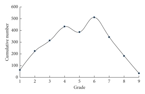
After the evaluation, Spearman correlation analysis between the rating results and the evaluators was carried out, and 8% of the unreliable data were removed. The distribution of evaluation results is shown in Figure 5. Most of the sample scores were within the range of 4–7 points, i.e., the grades ranged from “satisfactory” to “poor” in the subjective evaluation of sound quality.

4.2. Psychoacoustic Parameter Processing of Noise Samples

The psychoacoustic parameters [14] of the noise samples mainly included 8 parameters, which were the A-weighted sound pressure level (hereinafter referred to as A sound level), loudness, impulsiveness, sharpness, tonality, roughness, fluctuation strength, and articulation index (AI index). To reduce the complexity and training time of the BP neural network, the Pearson correlation analysis method was used to obtain the correlation distribution between the psychoacoustic parameters and evaluation score, as shown in Figures 6–9.

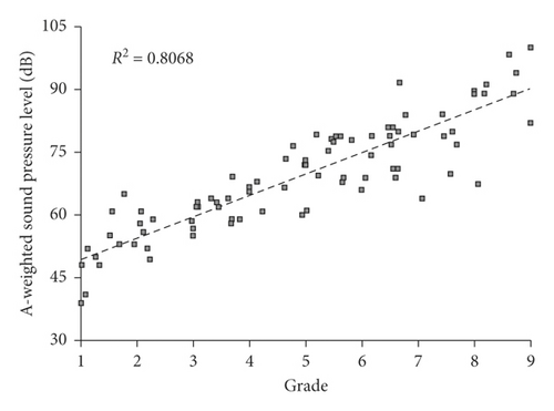
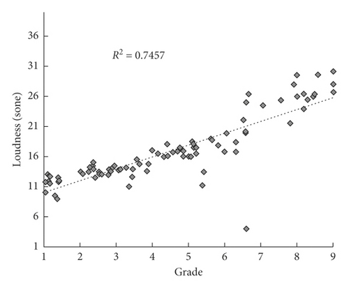
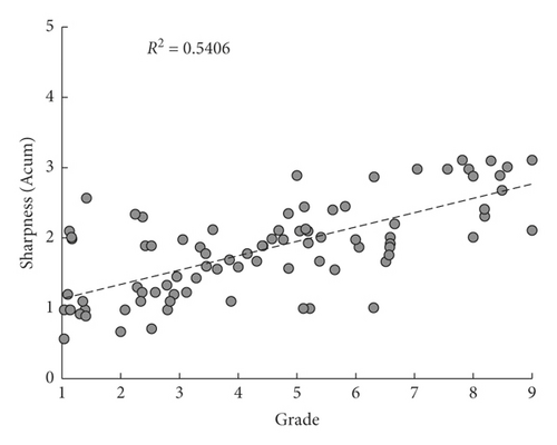
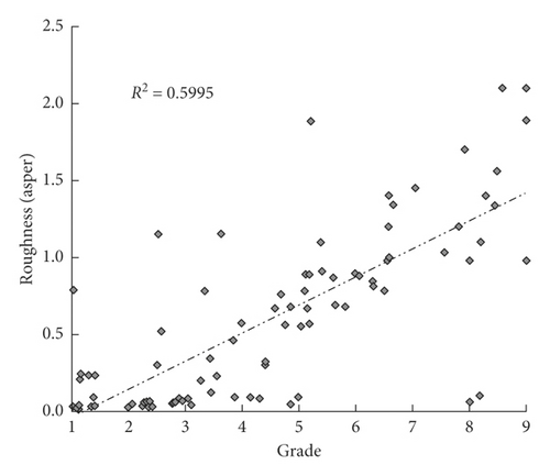
The correlation fitting curve shows that the correlation coefficients of the four parameters, i.e., A sound level, loudness, sharpness, and roughness, with the evaluation score were all more than 0.70. Table 1 shows that the correlation coefficients of the fluctuation strength and impulsiveness with the evaluation score were 0.563 and 0.346, respectively. The correlation significance <0.05 indicates that both the fluctuation strength and impulsiveness were linearly correlated to the evaluation score, but the correlation was insignificant. The correlations of the tonality and AI with evaluation score were less than 0.31, which indicated that the two parameters were not correlated to the evaluation score. The main reason was that the vibration noise of the vehicle’s internal combustion engine was insensitive to the sound quality, and the pitch values of internal combustion engines were not highly discriminated at different rotational speeds. Given the complexity of the BP model, training time, and the correlations between the objective parameters and evaluation score, four parameters, A sound level, loudness, sharpness, and roughness, were selected as the input variables of BP neural network.

Table 1. Correlation between psychoacoustic parameters and evaluation score.

Parameters	Correlation coefficient
A sound level	0.898 ^∗∗
Loudness	0.863 ^∗∗
Sharpness	0.735 ^∗∗
AI	0.392 ^∗
Tonality	0.282
Fluctuation strength	0.563 ^∗
Impulsiveness	0.386 ^∗
Roughness	0.774 ^∗∗

^∗∗P < 0.01; ^∗P ≤ 0.05, two-tailed.

4.3. BP Neural Network Structure

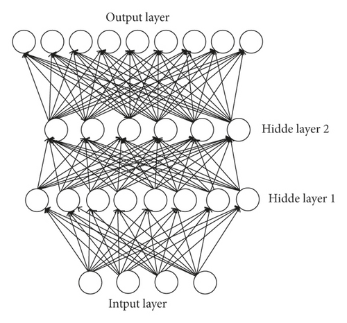
The topological structure of the BP neural network in this experiment consisted of four layers: an input layer, hidden layer 1, hidden layer 2, and output layer, as shown in Figure 10.

There were four nodes in the input layer in total, corresponding to four input psychoacoustic parameters. The number of nodes in the hidden layer was determined using the dropout method. After many trials, it was determined that there were eight nodes in hidden layer 1 and six nodes in hidden layer 2. The output layer had nine nodes, to match the levels of rating. The inputs and outputs of the hidden layers are expressed as follows:

\begin{matrix} h i_{l} (k) = \sum_{i = 1}^{n} w_{i l} x_{i} (k) - b_{l}, l = 1,2,3 \dots, p, \end{matrix}

(10)

where hi_l(k) denotes the input of the k^th sample in layer l and w_il denotes the weight of the i^th node in layer 1, and

\begin{matrix} {ho}_{l} (k) = f (h i_{l} (k)), l = 1,2,3, \dots, p, \end{matrix}

(11)

where ho_l(k) denotes the output of the k^th sample in layer l and f(x) denotes activation function:

\begin{matrix} f (x) = \frac{e^{x} - e^{- x}}{e^{x} + e^{- x}} . \end{matrix}

(12)

4.4. BP Neural Network Training

The data of the four psychoacoustic parameters of 80 sound samples were selected as training samples, and the remaining 10 were used as test samples. The algorithm of the normalizing variables before the input is shown in equation (16) below. The average error E_avg of the model classification and training is expressed as follows:

\begin{matrix} E_{avg} = \frac{1}{m} \sum_{i = 1}^{m} |y_{i} - y (x_{i})|, \end{matrix}

(13)

where y_i denotes the i^th expected output value, y(x_i) denotes the i^th calculated output value, and m denotes the number of samples.

The initial weight in the network model was generated randomly using the Nguyen–Widrow algorithm as follows:

\begin{matrix} w = 0.7 n^{1 / r} * random (n, r), \end{matrix}

(14)

where n denotes the number of neurons in each layer, which are n₁ = 4, n₂ = 8, and n₃ = 6, and r denotes the dimension of input vector, which was set to 4 in this experiment. To avoid the problem of local optimal solutions arising from the gradient descent method used in the training, the simulated annealing arithmetic algorithm [15] (SAA) was used. In this algorithm, if the objective function value of current state x was less than that of state x₁, then x₁ was accepted as the optimal point. Otherwise, the acceptance probability p = exp((f(x) − f((x₁))/t) was calculated. If p > random (0, 1), then x₁ was accepted as the optimal point. The initial temperature was 1000°C. The temperature attenuation rate was 0.7. The learning rate in the training was 0.03. The training iteration was carried out 4500 times, and the target error was set to 0.008.

5. Sound Quality Evaluation Based on the Auditory Model

The sound samples collected in Section 4.1 were used in the auditory model test. The input sound signals were processed using the time domain signal and auditory spectrum [8], respectively. The CNN model was used for comparison.

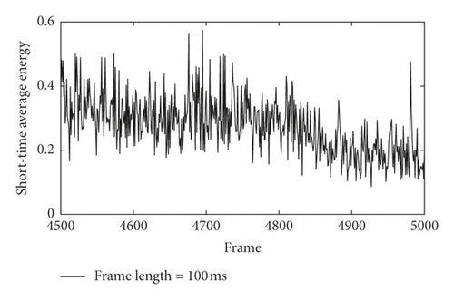
5.1. Time-Domain Signal Processing of Noise Samples

The intensity of the noise signal in different time periods was described using the short-time average energy, which reflected the energy information of the sample signal. This could be used for determining the time domain eigenvalues of sound signals, e.g., noise contrast or noise and mute distinction. In this transformation, the values of each sampling point in a short time frame were squared, and the time series consisting of short-time energy through an impulse function (window function) was output. The equation for this calculation is as follows:

\begin{matrix} E_{m} = \frac{1}{N} \sum_{m} {[x (n) w (n - m)]}^{2}, \end{matrix}

(15)

where E_m denotes the average energy of the m^th short frame, time-domain signal x(n) denotes the value of the n^th sampled signal in the m^th short frame signal, and W(n) denotes the window function with length N. A Hamming window function was used, and α was set to 0.46. Sampling was carried out at a frame size interval of 100 ms, and the frame offset was 20 ms. The short-time average energy fragments (4500–5000 frames) of the sample signals were calculated, as shown in Figure 11.

5.2. Auditory Spectrum Transformation of Noise Samples

The proposed auditory model based on gammatone filter banks was used for the auditory spectrum transformation. The overlapping segmentation method was used for signal processing. During downsampling, the filter response y(t, s) of each frequency channel was windowed at an interval of 100 ms frame size and an offset of 10 ms. A 64 × 100 matrix representing the time-frequency domain of input signal was thereby obtained. Its spectrum is shown in Figure 12.

To ensure a fast convergence speed of the model training, the input data used should be normalized. The normalized equation for the noise samples is as follows:

\begin{matrix} x = \frac{x_{i} - x_{\min}}{x_{\max} - x_{\min}} . \end{matrix}

(16)

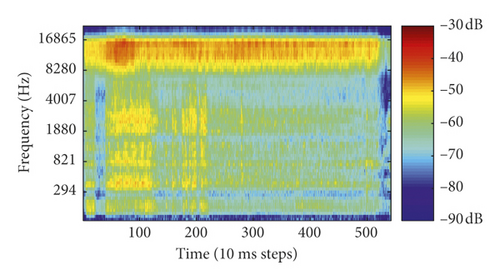
The output label value of the CNN model is the grade vector representation of the subjective evaluation results on a scale of 1 to 9.

5.3. Structure of Convolutional Neural Network

In the CNN model, the first layer was the input layer, followed by a three-layer convolution and three-layer pooling alternately. Next, there was the fully connected layer, followed by the Softmax classifier [16]. The detailed structure is shown in Table 2.

Table 2. Structure of convolutional neural network evaluation model.

Layer	Type	Structure (quantity × row × column)	Description
Conv1-64	Convolution layer	64 × 7 × 7	64 convolution kernels of size 7 × 7
MaxPooling	Pooling layer	3 × 3	Pool size 3 × 3
Conv2-128	Convolution layer	128 × 5 × 5	128 convolution kernels of size 5 × 5
MaxPooling	Pooling layer	3 × 3	Pool size 3 × 3
Conv3-256	Convolution layer	256 × 3 × 3	256 convolution kernels of size 3 × 3
MaxPooling	Pooling layer	3 × 3	Pool size 3 × 3

5.4. Training and Optimization

To ensure the comparability of test results, in the evaluation based on the CNN model, Conv1-64 in Table 2 was used in the input signal experiment for the first layer convolution (pad = 1, stride = 1), and a 3 × 3 pooling layer (pad = 1, 0, stride = 2) was used for the maxpooling to obtain 64 × 30 × 48 output feature map. In the second convolution layer, Conv2-128 (5 × 5, pad = 1, stride = 1) and the maxpooling window were used to generate a 128 × 14 × 23 feature map. In the third convolution layer, Conv3-256 (3 × 3, pad = 1, stride = 2) and the same pooling window were used to complete the convolution operation and output 256 × 3 × 6 eigenvalues. In the fourth layer, i.e., the fully connected layer, there were 4608 explicit nodes and 300 hidden nodes. Finally, the predictive probabilities for nine kinds of noise qualities were output by connecting the Softmax classifier.

The random initialization algorithm proposed in Section 4.4 was also used to initialize the weights in the CNN. In the training experiment, 10 samples were selected for each batch to predict the gradient and 60 iterations were performed for each batch. To accelerate the convergence, batch normalization was applied to the output of each layer. The adaptive moment estimation (Adam) algorithm [17] was used for training gradient descent optimization. The Adam algorithm could calculate the adaptive learning rate of each parameter. It preserved not only the exponential attenuation average of the square gradient but also the exponential attenuation average of the previous gradient M(t). Thus, it could be used to deal with the sparse gradient problem of convex functions quickly. The learning rate was set to 0.01. To prevent overfitting, 50% of the nodes were randomly removed or 30% of the hidden layer nodes were randomly removed in each batch of training in the fourth layer.

6. Results and Analysis

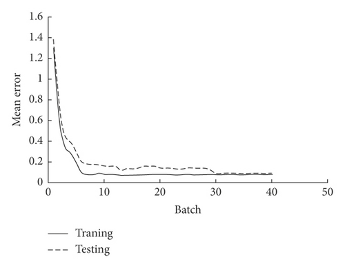
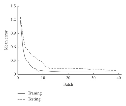
Figure 13 shows the trends of the training and test losses of the auditory spectrum input in the CNN evaluation test. The loss tended to be stable after 5300 iterations, indicating that the model converged and no overfitting occurred. Noise was added randomly to the sample, and dropout technology was used to prevent overfitting, which showed that the robustness of the classification model increased. Figure 14 shows the trends of the training and test losses in the BP evaluation test. After 4500 training iterations, the model converged without underfitting or overfitting.

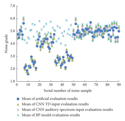
As shown in Figure 15, the x-axis represents the serial number of noise sample and the y-axis means the noise grade. Different types of points in the graph show the mean of multiple evaluation results for different models. The coincidence degree of the evaluation average based on the CNN auditory spectrum input and artificial evaluation average was the highest, and the coincidence degree of the evaluation average based on the CNN time and frequency domain inputs and artificial evaluation average was higher than that of BP model.

The overall accuracy and error are shown in Tables 3 and 4. Variable A represents the weighted sound pressure level. Input variable L represents the loudness, and variables R and S represent the roughness and sharpness, respectively. The accuracy of the auditory spectrum input training in the CNN model was 97.31%, and the testing accuracy was 95.28%. Compared to the control model, i.e., the BP neural network evaluation model, the accuracy of the CNN model was at most 5.95% higher. In the CNN evaluation model, the accuracy of the auditory model input was 3.53% higher than that of the time domain input. The single input results in the CNN model obtained using loudness, roughness, and sharpness showed that the input had no obvious advantages in the classification accuracy of the sound quality. The results also showed that the convolution neural network possessed strong automatic feature extraction and expression abilities. It could accurately express the features of the samples when the samples were input with complete time-frequency information and achieve good classification. Furthermore, because the convolution operation had sparse features of the sample signal expression, the complexity of the training was effectively reduced by features such as parameter sharing.

Table 3. Comparison of test results of two evaluation models.

Model	Input	Training accuracy (%)	Test accuracy (%)
CNN	Auditory spectrum	97.31	95.28
CNN	L	90.25	89.13
CNN	R	88.58	87.47
CNN	S	88.22	87.13
CNN	A	90.25	89.56
BP	L, R, S, A	90.11	89.33

Table 4. Comparison of auditory spectrum and time-domain input test results.

Model	Input	Training accuracy (%)	Test accuracy (%)
CNN	Auditory spectrum	97.31	95.28
CNN	Time domain	92.79	91.75

7. Conclusions

(1)
In this study, an auditory model-based automatic evaluation method was proposed to evaluate the sound quality of internal combustion engines. The hierarchical structure of a CNN and the size and thickness of the convolution kernel were designed. The sound samples collected in the evaluation were used to obtain a time-frequency auditory spectrum simulating the auditory characteristics of the human ear basement membrane through gammatone filter banks. The input was used to train the CNN model, which could accurately express the characteristics of the samples and achieve good evaluation and classification.
(2)
The training accuracy of the auditory spectrum input in the CNN model was much higher than that of the BP neural network evaluation model, and the time domain input test results of the CNN evaluation model also indicated better performance than that of the BP neural network evaluation model. Therefore, the CNN evaluation model was a better evaluation model for the classification of internal combustion engine sound quality.
(3)
The experiments of 20 groups of different types of newly collected internal combustion engine sound samples showed that the proposed model has good generalization abilities. It was compared with CNN experiments using frequency domain and time domain inputs. The results showed that the sound quality classification method based on an auditory model was effective.

Conflicts of Interest

The authors declare that they have no conflicts of interest.

Open Research

Data Availability

The data used to support the findings of this study are available from the corresponding author upon request.

References

1 Meng X., Zhang J., and Li L., Sound quality prediction of diesel engine noise based on regression analysis, Transactions of CSICE. (2011) 29, no. 6, 534–537.
Google Scholar
2 Xu Z., Zhang Y., and Liu J., Sound quality analysis of wiper system noise in cars, Automotive Engineering. (2014) 36, no. 8, 1009–1013.
Google Scholar
3 Huang H., Huang X., and Su R., Sound metric prediction of a power train system based on EEMD and GA-wavelet neural network, Journal of Vibration and Shock. (2017) 36, no. 9, 130–137.
CAS Google Scholar
4 Wu L. and Yang H., Application of auditory spectrum features into echo target recognition, Ship Science and Technology. (2016) 38, no. 23, 143–146.
Google Scholar
5 Wu W., Li Y., Wang B., Li G., and Shi Y., A method extracting fault features of gear teeth fractures based on an auditory modeland probability density of extreme points, Journal of Vibration and Shock. (2016) 35, no. 19, 101–106.
Google Scholar
6 Liang J., Research on analysis and evaluation method of vehicle interior sound quality based on binaural auditory model, 2007, Jilin University, Changchun, China, Ph.D. thesis.
Google Scholar
7 Klaus F., Rainer M., and Claus W., A computational study of auditory models in music recognition tasks for normal-hearing and hearing-impaired listeners, EURASIP Journal on Audio, Speech, and Music Processing. (2017) 2017, no. 1, 13636–13658, https://doi.org/10.1186/s13636-017-0103-7, 2-s2.0-85014595374.
10.1186/s13636-017-0103-7
Google Scholar
8 Li Y., Zhang J., and Dai L., Auditory spectrum of mechanical vibration signal and its characteristics, Journal of vibration and shock. (2010) 29, no. 11, 204–208.
Google Scholar
9 Li Y., Zongbo H., and Lei H., Survey of convolutional neural network, Journal of Computer Applications. (2016) 36, no. 9, 2508–2515.
Google Scholar
10 Pan X. and Srikumar V., Expressiveness of rectifier networks, 2016, https://arxiv.org/pdf/1511.05678.
Google Scholar
11 Lecun Y., Bottou L., Bengio Y., and Haffner P., Gradient-based learning applied to document recognition, Proceedings of the IEEE. (1998) 86, no. 11, 2278–2324, https://doi.org/10.1109/5.726791, 2-s2.0-0032203257.
10.1109/5.726791
Web of Science® Google Scholar
12 Hinton G. E., Osindero S., and Teh Y.-W., A fast learning algorithm for deep belief nets, Neural Computation. (2006) 18, no. 7, 1527–1554, https://doi.org/10.1162/neco.2006.18.7.1527, 2-s2.0-33745805403.
10.1162/neco.2006.18.7.1527
PubMed Web of Science® Google Scholar
13 Lee H., Grosse R., and Ranganath R., Convolutional deep belief networks for scalable unsupervised learning of hierarchical rep-resentations, Proceedings of the 26th Annual Inter-national Conference on Machine Learning, 2009, ACM, New York, NY, USA, 609–616.
Google Scholar
14 Qian K., Evaluation and control technology of sound quality of electric vehicles, 2016, Jilin University, Changchun, China, Ph.D. thesis.
Google Scholar
15 Lowe D. G., Object recognition from local scale-invariant features, Proceedings of the 7th IEEE International Conference on Computer Vision, September 1999, Kerkyra, Greece, IEEE Press, 1150–1157.
Google Scholar
16 Dalal N. and Triggs B., Histograms of oriented gradients for human detection, l, Proceedings of IEEE Computer Society Conference on Computer Vision and Pattern Recognition, June 2005, San Diego, CA, USA, IEEE Press, 886–893.
Google Scholar
17 Shen L. and Li B., A review on gabor wavelets for face recognition, Pattern Analysis and Applications. (2006) 9, no. 2-3, 273–292, https://doi.org/10.1007/s10044-006-0033-y, 2-s2.0-33749335686.
10.1007/s10044-006-0033-y
Web of Science® Google Scholar
18 Tan X. and Triggs B., Enhanced local texture feature sets for face recognition under difficult lighting conditions, IEEE Trans on Image Processing. (2010) 19, no. 6, 1635–1650, https://doi.org/10.1109/tip.2010.2042645, 2-s2.0-77952634397.
10.1109/TIP.2010.2042645
PubMed Web of Science® Google Scholar
19 Guo Z., Zhang L., and Zhang D., A completed modeling of local binary pattern operator for texture classification, IEEE Trans on Image Processing. (2010) 19, no. 6, 1657–1663, https://doi.org/10.1109/tip.2010.2044957, 2-s2.0-77952607168.
10.1109/TIP.2010.2044957
PubMed Web of Science® Google Scholar

Citing Literature

All articles

Automatic Evaluation of Internal Combustion Engine Noise Based on an Auditory Model

Abstract

1. Introduction

2. Auditory Model