Volume 2019, Issue 1 2015465
Research Article
Open Access

Formulation of a Linearized Model for Vehicle-Track Interactions

Fei Huo

Corresponding Author

Fei Huo

State Key Laboratory of Traction Power, Southwest Jiaotong University, Chengdu 610031, China swjtu.edu.cn

Search for more papers by this author
Huanyun Dai

Huanyun Dai

State Key Laboratory of Traction Power, Southwest Jiaotong University, Chengdu 610031, China swjtu.edu.cn

Search for more papers by this author
Academic Editor: Miguel Neves

Abstract

In this paper, a fundamental wheel-rail interaction (WRI) element accompanied by its coupling matrices with other vehicle-track components have been derived taking into consideration the aspect of linearization. The key to the presented formulation is the use of the geometrical relationships of relative motions between degrees of freedom (DOFs) and energy principle. To the WRI element, both of the conditions of wheel-rail contacts and wheel-rail separations are allowed in the numerical computations; besides, the effects of the linear creepage and the gravitational restoring are considered in the description of wheel-rail interactions. By comparing with an advanced three-dimensional nonlinear model, the capability of the linear model in characterizing the response amplitude and frequency characteristic of vehicle-track systems is demonstrated. Moreover, the method for the random vibration analysis of the linear model is presented by treating the creep coefficients as the random sources, through which the safety margin of system response can be predicted well. From the numerical examples, it is, additionally, concluded that the lateral creep coefficient holds significant influence on wheel-rail lateral interactions and track vibrations, especially for the responses at low frequency ranges.

1. Introduction

To ensure a comfortable, safe, and efficient transportation, it was critical to scientifically assess the dynamic performance of vehicle-track systems under varying loads; consequently, a vehicle-track interaction system was formulated. The vehicle-track interactions are essentially nonlinear, while for lowering the modelling complexity, increasing the computational efficiency, and broadening the model application, it was rather popular to simplify the vehicle-track systems as a coupled and linearized system.

In the last decades, the models aiming at describing the vehicle-track interactions have experienced a rapid development from the earliest two-dimensionally vertical models [18] to more advanced three-dimensionally spatial ones. Concerning the system nonlinearity, Sun et al. [9] presented a 3D wagon-track system dynamics model, where a wagon system with 37 degrees of freedom (DOFs), a four-layer track, and the wheel-rail interfacial contacts were comprehensively considered; Zhai et al. [10] presented a theoretical framework and methodologies for characterizing the 3D nonlinear vehicle-track interactions; recently, Xu and Zhai [11, 12] made pioneering and the most advanced work in developing temporal-spatial stochastic models for train-track (bridge) interactions, in which the finite element method (FEM) and random theory were introduced to construct the track systems and to achieve the random vibration analysis, respectively.

With the development of nonlinear models, the methodologies are constantly developed to mathematically investigate the vehicle-track (bridge) interactions in the field of linearization modelling. See for instance, Zeng and Guo [13] made pioneering work on building a train-bridge time-dependent model by an application of the principle of a stationary value of total potential energy of dynamic system [14]; Yang and Wu [15] proposed a versatile element that is capable of considering various vehicle-bridge interaction (VBI) effects; however, the condition of wheel-rail separation is neglected in both of the these two models. Some other related researches can be consulted in [16, 17]. Moreover, Zhang et al. [18] regarded the vehicle as a spring-mass-damper system and the track as an infinitely long substructural chain consisting three layers of rail, sleeper, and ballast, and the vehicle and the tracks were coupled by linear springs; based on this developed model, the pseudoexcitation method (PEM) was introduced to achieve the high-efficient frequency characteristic analysis for system indices. Nguyen et al. [19] presented simulations for vehicle-substructure dynamic interactions and wheel movements, where the two compatibilities, i.e., force equilibrium and geometrical relation, are satisfied in the wheel-rail interfaces.

Additionally, the train-track dynamic simulations under transient conditions also show remarkable significance to railway maintenance, assessment, rolling fatigue, safety, etc. See for instance, Handoko and Dhanasekar [20] pointed out that the traction and braking forces are seldom considered in the practice of wagon dynamics simulation, although these forces will greatly modify the wheel-rail contact parameters and then the wheelset dynamics; Liu et al. [21] also studied the mechanism of wheelset longitudinal vibration by analysing the process of wheel/rail rolling contact; generally, the track defects can cause profound effects to the dynamics of the railway wagon; Zhang and Dhanasekar [22] noticed this problem and published a model for the dynamics of wagons subject to braking/traction torques on a perfect track by explicitly considering the pitch degree of freedom for wheelsets [23, 24] and extended this model for cases of lateral and vertical track geometry defects and worn railhead and wheel profiles; Grossoni et al. [25] examined the dynamic behaviour at a rail joint using a two-dimensional vehicle-track coupling model, where the influence of the number of layers and the number of elements between two sleepers and the beam model are investigated. Laterally, Zong and Dhanasekar [26] considered the gap between rail joints to account for thermal movement and to maintain electrical insulation for the control of signals and/or broken rail detection circuits; besides, railhead can provide high stresses due to the passage of heavily loaded wheels through a very small contact patch [27], and a multibody dynamic model was developed in [28] to accurately model and analyse the track dynamic behaviour in vicinity of rail discontinuities; recently Zong and Dhanasekar [29] provided a idea of simplifying the design of the IRJs consisting of only two pieces of insulated rails embedded into a concrete sleeper; Ling et al. [30] presented a formulation for a passive road-rail crossing involving stiffened edges of the raised road pavement to minimise the risk of failure of wheel-rail contact using a nonlinear three-dimensional multibody dynamics model; additionally, a series of work on impact derailment due to lateral collisions between heavy road vehicles and passenger trains at level crossings and the associated derailments had also been conducted in [3134].

In the above presentations, though the nonlinear and linear vehicle-track interaction, models have been established by many researchers, while the applicability of the linear model and its comparison to the nonlinear model have rarely been reported. In this paper, a contribution, which is not beneficial to train-track dynamic to severe transient impact/rolling issues, was made to develop a highly practical and efficient model, and fully deriving the equation of motion for the linearized vehicle-track interactions. The coupling mechanism between a railway vehicle and the tracks in relation to wheel-rail interactions and system responses that are of great interest to railway engineers will be revealed.

The organization of this paper is listed as follows:
  • (1)

    In section 2, a general wheel-rail interaction (WRI) element is presented, in which the jumping of the vehicle off the rail, the linear creepage, and gravitational restoring actions are properly considered.

  • (2)

    In section 3, the coupling matrices for building the physical-mechanical connections between system components and WRI element are elaborately illustrated and finally the unified equation of motion for the vehicle-track system is established.

  • (3)

    In section 4, numerical examples, including comparisons with the nonlinear model and a practice of random vibration analysis, are conducted to validate the reliability and feasibility of the proposed model.

  • (4)

    In section 5, some conclusions are drawn accordingly.

2. WRI Element

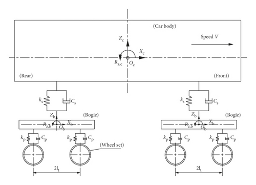
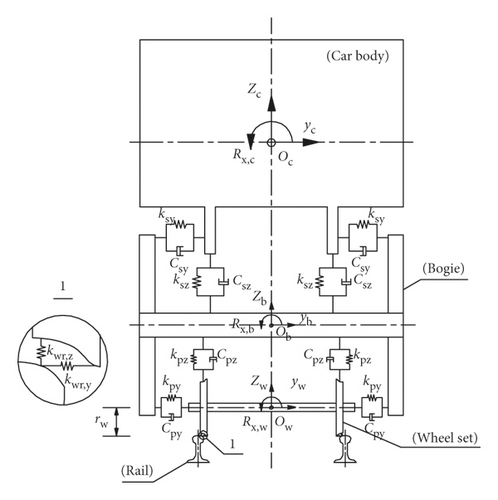
In the whole vehicle-track model presented in Figure 1, the wheel-rail interactions play a key role in determining the dynamic trajectories of vehicle/track behaviours. In this part, a wheel-rail interaction (WRI) element will be developed to depict the wheel-rail interaction mechanism from aspect of linearization.
Details are in the caption following the image
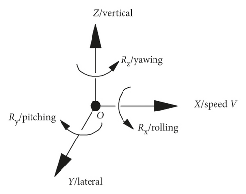
Model, dimensions, and parameters of a vehicle. (a) Side view; (b) front view; (c) top view; (d) sign convention of degree of freedoms.
Details are in the caption following the image
Model, dimensions, and parameters of a vehicle. (a) Side view; (b) front view; (c) top view; (d) sign convention of degree of freedoms.
Details are in the caption following the image
Model, dimensions, and parameters of a vehicle. (a) Side view; (b) front view; (c) top view; (d) sign convention of degree of freedoms.
Details are in the caption following the image
Model, dimensions, and parameters of a vehicle. (a) Side view; (b) front view; (c) top view; (d) sign convention of degree of freedoms.

2.1. Displacement Vector

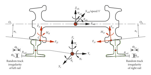
For a wheel-rail contact pair, as shown in Figure 2, the displacement vector, X ˜ wr, k , with order of T ˜ wr × 1 , can be expressed by
X ˜ wr, k = x w , k y w , k z w , k ψ w , k L v , k R v , k L z , k R z , k L h , k R h , k L y , k R y , k L n , k R n , k L x , k R x , k T , ()
where the superscript “T” denotes the transposition of vectors or matrices; the subscript “k” denotes the kth wheel-rail contact element; xw, yw, zw, and ψw are the longitudinal, lateral, vertical, and yaw motions of the wheel; by assuming the track irregularity as virtual displacement of the rail at the wheel-rail contact positions, Lv and Rv are the vertical irregularities of the rail at the left and right side, respectively, Lh and Rh are the lateral irregularities of the rail at the left and right side, respectively; moreover, Lz and Rz, respectively, denote the vertical displacement of the left- and right-side rail at the wheel-rail contact points; in the same manner, Ly and Ry denote the lateral displacement of the left- and right-side rail at the wheel-rail contact points, respectively; Ln and Rn denote the angle of torsion of the left- and right-side rail around the Y axis, respectively; and Lx and Rx denote the longitudinal displacement of the rails with respect to the left and right wheel-rail contact points, respectively.
Details are in the caption following the image
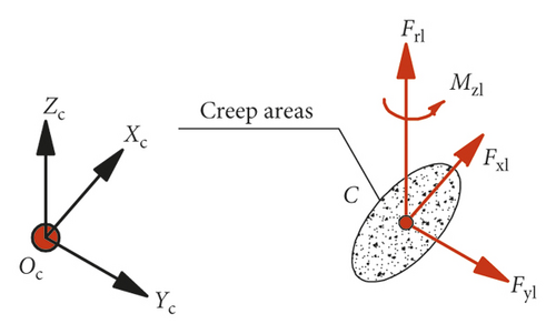
3D random wheel/rail contact model: (a) front view; (b) elliptical contact spot at location of C.
Details are in the caption following the image
3D random wheel/rail contact model: (a) front view; (b) elliptical contact spot at location of C.
In normal wheel-rail contacts, it is assumed that the vertical motion of the wheel is nonindependent and being totally determined by the rail vertical displacement, namely,
z w , k = 1 2 L v , k + R v , k + L z , k + R z , k , ()
with
L z , k = D R , z l, k N R , z , k T , R z , k = D R , zr, k N R , z , k T , D R , zl, k = W R 1 , l θ R 1 , ly W R 2 , l θ R 2 , ly , D R , zr, k = W R 1 , r θ R 1 , ry W R 2 , r θ R 2 , ry , N r , 1 = 132 ζ w , k / l wr 2 + ζ w , k / l wr 3 , N r , 2 = ζ w , k 12 ζ w , k / l wr + ζ w , k / l wr 2 , N r , 3 = 32 ζ w , k / l wr 2 ζ w , k / l wr 3 , N r , 4 = ζ w , k ζ w , k / l wr 2 ζ w , k / l wr , N R , z , k = N r , 1 N r , 2 N r , 3 N r , 4 , ()
where DR,zl and DR,zr are the nodal displacement vector used to calculate the vertical displacement of the rail beam at the left and right side along the X axis; W and θy are the nodal vertical displacement and angular displacement of the node around the Y axis, in which the subscripts “l” and “r” denote the left- and right-side rails, respectively and the subscripts “R1” and “R2” denote the left and right nodes with respect to the rail beam element, respectively; ζw denotes the distance between the left node of the rail element and the wheel-rail contact position; and NR,z is the Hermite polynomial interpolation used for Euler–Bernoulli beam.
When the wheels lose contact with the rails, the vertical motion of the wheel is independent, by assuming zw in Equation (1) as an independent degree of freedom (DOF). In the numerical simulation, the inequalities below are applied to judge whether or not the wheelsets are contacting to the rails [35] (set the left wheel-rail contact side as an example):
L v + L z z w min L v + L z , z w < ξ 1 , 11 ξ 2 L v + L z z w , when z w > 0 , L v + L z > 0 , 11 ξ 3 z w L v + L z , when z w < 0 , L v + L z < 0 , max L v + L z , z w ξ 4 , when z w < 0 , L v + L z > 0 , ()
where ξi, i = 1,2,3,4, is a small positive number depending on the analytical precision.

2.2. Wheel-Rail Coupling Matrices

In most of the running conditions, the wheels constantly keep contact with the rails, thus the wheel-rail coupling matrices that consider the wheelset’s vertical displacement as nonindependent will be presented here as an emphasis. The wheel-rail coupling matrices are marked by subscript “wr” with order of T ˜ wr × T ˜ wr .

The mass submatrix of WRI element can be written as
M ˜ wr = k = 1 n wr M wr, k Θ m , k , Θ m , k + M wr, k x w , k , x w , k + M wr, k y w , k , y w , k + M wr, k ψ w , k , ψ w , k , = k = 1 n wr m w , z , k N m T N m + m w , y , k + m w , x , k + I w z , k , ()
with N m = 12 / 12 / 12 / 12 / , where mw,z, mw,y, and mw,x denote the mass of the wheelset against the vertical, lateral, and longitudinal motion of the wheelset; Iwz is the mass moment of inertia of the wheelset around the Z axis; Θm is the number of the freedoms in Equation (1) related to the mass submatrix, Θ m = L v R v L z R z , [⋅] denotes the operator characterizing the corresponding number of DOF in the displacement vector, and nwr = 4 for a four-axle vehicle.
The damping submatrix of WRI element is mainly induced by the virtual work of wheel-rail creep forces, which can be derived as
C ˜ wr = k = 1 n wr C wr , 1 l, k Θ c , 1 l, k , Θ c , 1 l, k + C wr , 1 r, k Θ c , 1 r, k , Θ c , 1 r, k + C wr, 2 l, k Θ c , 2 l, k , Θ c , 2 l, k + C wr, 2 r, k Θ c , 2 r, k , Θ c , 2 r, k = k = 1 n wr C X V ¯ N c 1 , l T N c 1 , l + N c 1 , r T N c 1 , r + C Y V ¯ N c 2 , l T N c 2 , l + N c 2 , r T N c 2 , r , ()
with
N c 1 , l = 1 l lr 1 , N c 1 , r = 1 l lr 1 , N c 2 , l = 1 1 1 l cp , N c 2 , r = 1 1 1 l cp , Θ c , 1 l, k = x w , k ψ w , k L x , k , Θ c , 1 r, k = x w , k ψ w , k R x , k , Θ c , 2 l, k = y w , k L h , k L y , k L n , k , Θ c , 2 r, k = y w , k R h , k R y , k R n , k , ()
where CX and CY denote the longitudinal and lateral creep coefficient, respectively; V ¯ is the forward speed of the wheelset nominally; Cwr,1l and Cwr,1r denote the damping matrices derived by the virtual work of wheel-rail longitudinal creep forces; Cwr,2l and Cwr,2r denote the damping matrices derived by the virtual work of wheel-rail lateral creep forces; llr is the lateral half distance the two wheel-rail contact points at the left and right side, and lcp is the vertical distance between the wheel-rail contact point and the centroid of the wheelset.
The stiffness submatrix of WRI element is mainly derived from the work of wheel-rail equivalent gravity stiffness, namely,
K ˜ wr = k = 1 n wr K wr , k Θ s , k , Θ s , k = n = 1 n wr k g , k N s , k T N s , k , ()
with
Θ s , k = y w , k L h , k R h , k L y , k R y , k , N s , k = 1 12 / 12 / 12 / 12 / , ()
where kg,k is the wheel-rail equivalent gravity stiffness, which is calculated using the following equation [36]:
k g = W b ϕ ς δ 0 + ε , ()
with
ε = b R R ϕ 1 1 + R δ 0 b , ς = R R R ϕ 1 1 + R δ 0 b , ϕ 1 = 1 r 0 δ 0 b , ()
where ε is the angular parameter of the wheel-rail contact, ς is the change rate of the lateral relative displacement between the wheel centroid and wheel-rail contact point, b is the half of lateral distance between two rolling circles, R and R are the radii of curvature of the wheel and the rail at the contact point, respectively, δ0 is the wheel-rail contact angle when the wheelset is placed in the central position, and r0 is the radius of the nominal rolling circle.
The load vector of WRI element is originated from the gravity of the wheelset, namely,
F ˜ wr = k = 1 n wr F wr, k Θ f l, k , Θ f l, k + F wr, k Θ f r, k , Θ f r, k = k = 1 n wr 1 2 m w , k g N f l + 1 2 m w , k g N f r , ()
with
Θ f l, k = L v , k L z , k , Θ f r, k = R v , k R z , k , N f l = N f r = 1 1 , ()
where g is the gravitational acceleration.
Equations (5), (6), and (8) have briefly presented the mass, damping, and stiffness matrices of WRI element, namely, M ˜ wr , C ˜ wr , and K ˜ wr all with order of n wr T ˜ wr × n wr T ˜ wr . Moreover, it should be noted that the some of the DOFs in Equation (1), i.e., Lz,k, Rz,k, Ly,k, Ry,k, Ln,k, Rn,k, Lx,k, and Rx,k, which can be called as the interior node, are the interpolation results of the nodal displacements of the rail beam element. Besides L z , k = D R , z l N R , z T and R z , k = D R , z r N R , z T illustrated in Equation (2), the other DOFs can be equivalently transformed by the nodal displacement as
L y , k = D R , y l N R, y T , R y , k = D R , y r N R, y T , ()
with
D R , y l = V R 1 ,l θ R 1 ,l z V R 2 ,l θ R 2 ,l z , D R , y r = V R 1 ,r θ R 1 ,r z V R 2 ,r θ R 2 ,r z , N R, y = N r , 1 N r , 2 N r , 3 N r , 4 , ()
where V denotes the lateral displacement of the rail node, θz denotes the angular displacement of the rail node around the Z axis.
Moreover,
L n , k = D R , n l N R, n T , R n , k = D R , n r N R, n T , ()
with
D R , n l = θ R 1 ,l x θ R 2 ,l x , D R , n r = θ R 1 ,r x θ R 2 , r x , N R, n = 1 ζ w , k / l wr ζ w , k / l wr , ()
where θx denotes the angular displacement of the rail node around the X axis:
L x , k = D R , x l N R, x T , R x , k = D R , x r N R, x T , ()
with
D R , x l = U R 1 , l x U R 2 , l x , D R , x r = U R 1 , r x U R 2 , r x , N R, x = N R, n , ()
where Ux denotes the longitudinal displacement of the rail node.
Based on Equations (2), (14), (16), and (18), the displacement vector, X ˜ wr, k , presented in Equation (1) can be further extended as
X ˜ wr, k = x w , k y w , k z w , k ψ w , k T L v , k R v , k W R 1 ,l, k θ R 1 ,l y , k W R 2 ,l, k θ R 2 ,l y , k W R 1 ,r, k θ R 1 ,r y , k W R 2 ,r, k θ R 2 ,r y , k T L h , k R h , k V R 1 ,l, k θ R 1 ,l z , k V R 2 ,l, k θ R 2 ,l z , k V R 1 ,r, k θ R 1 ,r z , k V R 2 ,r, k θ R 2 ,r z , k T θ R 1 ,l x , k θ R 2 ,l x , k θ R 1 ,r x , k θ R 2 ,r x , k T U R 1 ,l x , k U R 2 ,l x , k U R 1 ,r x , k U R 2 ,r x , k T . ()
In the meantime, the dynamic matrices and load vector over WRI element can be conveniently redistributed into this extensive nodal displacement vector; for example, the newly developed mass matrix Mwr with order Twr × Twr can be obtained by
M wr = M ˜ wr Θ m , D R , z r + M ˜ wr Θ m , D R , z l + M ˜ wr D R , z r , Θ m + M ˜ wr D R , z l , Θ m , ()
with
M ˜ wr Θ m , D R , z r = M ˜ wr Θ m , R z N R , z , M ˜ wr Θ m , D R , z l = M ˜ wr Θ m , L z N R , z , M ˜ wr D R , z r , Θ m = N R , z T M ˜ wr R z , Θ m , M ˜ wr D R , z l , Θ m = N R , z T M ˜ wr L z , Θ m . ()

Using the same strategy, the damping matrix, stiffness matrix, and load vector over the extensive displacement vector, i.e., Cwr, Kwr, and Fwr, can be derived in the same way as Mwr.

3. Vehicle-Track Interaction Model

As illustrated in Figure 1, a ballastless track system was formulated with a moving vehicle subjected to constant velocity. The railway vehicle was modelled as a four-axle mass-spring-damper system, which consisted of a car body, two bogie frames, four wheelsets, and two stage suspensions. The car body and bogie frames have 6 DOFs each including motions of longitudinal X, transverse Y, bounce Z, roll Φ, yaw ψ, and pitch β with respect to their mass centroids, respectively, while for the wheelsets, only the motions of longitudinal, transverse, vertical, and yaw were considered. The total number of DOFs of vehicle system was therefore 34. The vehicle proceeded with velocity v in the longitudinal direction.

In the track system, the rails were modelled as spatial Bernoulli–Euler beam supported by discrete viscoelastic supported with finite length, and the rail pads were assumed as linear spring-damper elements. Moreover, slab tracks were assumed to be thin plate elements connected to subgrade through cement asphalt mortar (CA mortar) layer, which was regarded as continuous plane springs and dashpots.

3.1. Equation of Motion for the Vehicle-Track Interaction Systems

The wheel-rail coupling system had been formulated and characterized by dynamic matrices in Section 2, based on which one can derive the equation of motion written in submatrix form for the vehicle-track interaction systems by energy principle [13]:
M vv 0 0 0 M wr 0 0 0 M ss X ¨ v X ¨ wr X ¨ s + C vv C v wr 0 C wr v C wr C wr s 0 C s wr C ss X ˙ v X ˙ wr X ˙ s + K vv K v wr 0 K wr v K wr K wr s 0 K s wr K ss X v X wr X s = F v F wr F s , ()
where M, C, and K denote the mass, damping, and stiffness submatrices, respectively; X and F denote the displacement and force vectors, respectively; the subscripts “v,” “wr,” and “s” denote the vehicle, wheel-rail interaction element, and slab track, respectively.

The wheel-rail coupling matrices, namely, Mwr, Cwr, and Kwr, were core terms in Equation (23). In Equation (23), the elements in the wheel-rail coupling matrices can be partitioned and inserted into different positions based on the “set-in-right-position” rule [37]. The submatrices of the slab track accompanied by their interactions with the rail elements can be found in [38], here not given for brevity.

The submatrices of vehicle systems, the coupling submatrices between vehicle systems and wheel-rail interaction element and the force vectors will be elaborated in the following sections.

3.2. The “Set-in-Right-Position” Rule

It is assumed that there are totally n displacement parameters γi, i = 1, 2, …, n, and the total elastic potential energy is ∏(γi). Based on the total potential energy with stationary value, the first-order variation of ∏ is equal to zero, namely,
δ = i = 1 n γ i δ γ i = 0 , ()
and accordingly, there is
δ γ i γ i = 0 , i = 12… , , , n . ()

It is obvious that Equation (25) denotes the i-th equilibrium equation of this dynamic system. Herein, δγi denotes the i-th row in the matrix; besides, there are displacement parameters γj, j = 1, 2, …, n derived from ∏ /γi. In the dynamic matrices, the serial number j denotes the j-th column. Hence, the coefficient multiplied by δγi and γj should be set in the cross position of the matrix at the i-th row and the j-th column.

3.3. Matrices for the Vehicle Systems

The matrices of the vehicle were marked with the subscript ‘vv’. The mass matrix of the vehicle can be written as
M vv = M c Θ c , Θ c + M Gq Θ Gq , Θ Gq + M Gh Θ Gh , Θ Gh + k = 1 n wr M w , k Θ w , k , Θ w , k , ()
with
Θ q = x q y q z q ψ q β q ϕ q , M q Θ q , Θ q = diag m q m q m q I q , z I q , y I q , x , Θ w , k = x w , k y w , k ψ w , k , M w , k Θ w , k , Θ w , k = diag m w , k m w , k I w , z , k , ()
where x, y, z, ψ, β, and ϕ denote the longitudinal, lateral, vertical, yaw, pitch, and roll motions, respectively; the subscript “q” will be substituted by “c,” “Gq,” and “Gh” denoting the car body, front bogie frame, rear bogie frame, respectively; m denotes the mass; Ix, Iy, and Iz denote the moment of inertia of rigid-bodies around the X, Y, and Z axes, respectively.
The stiffness matrix of the vehicle can be written as
K vv = K sz 1 Θ sz 1 , Θ sz 1 + K sz 2 Θ sz 2 , Θ sz 2 + K sy 1 Θ sy 1 , Θ sy 1 + K sy 2 Θ sy 2 , Θ sy 2 + K sx 1 Θ sx 1 , Θ sx 1 + K sx 2 Θ sx 2 , Θ sx 2 , ()
where Ksz1, Ksy1, and Ksx1 denote the stiffness matrices induced by interactions between the car body and the front bogie frame in the vertical, lateral, and longitudinal directions, respectively; Ksz2, Ksy2, and Ksx2 denote the stiffness matrices induced by interactions between the car body and the rear bogie frame in the vertical, lateral, and longitudinal directions, respectively; Nsz, Nsy, and Nsx denote the equivalent shape functions used to characterize the geometrical relationships of the involved DOFs. The detail expressions of the parameters in Equation (28) are illustrated in Appendix A.

The damping matrix, i.e., Cvv, with the same order of Kvv, can be obtained by substituting the stiffness coefficient k in Kvv with damping coefficient c.

3.4. Matrices for the Vehicle-WRI Element Interactions

The coupling matrices for vehicle-WRI element interactions were marked with the subscript ‘v-wr’ or ‘wr-v’. Before deriving the matrices Kv−wr, Kwr−v, Cv−wr, and Cwr−v, one can deduce the interaction matrices between the vehicle and the rails at first, namely, Kvr and Cvr.

Kvr can be written as
K vr = K vr, z + K vr, y + K vr, x , ()
where the subscripts ‘z,’ ‘y,’ and ‘x’ denote the interactions between the bogies and the i-th wheelset in the vertical, lateral, and longitudinal direction, respectively. The details about the formation of these involved stiffness matrices have been presented in Appendix B.

The damping matrix, i.e., Cvr, with the same order of Kvr, can be obtained by substituting the stiffness coefficient k in Kvr with damping coefficient c.

The stiffness matrices Kvwr and Kwrv can be obtained by partitioning Kvr, that is,
K v wr = K vr Θ v , Θ wr , K wr v = K vr Θ wr , Θ v , ()
in which
Θ v = x Gp y Gp z Gp ψ Gp β Gp ϕ Gp x Gh y Gh z Gh ψ Gh β Gh ϕ Gh , Θ wr = x w , i y w , i ψ w , i L v , i R v , i L z , i R z , i . ()

The damping matrices Cv−wr and Cwr−v had the same expression as Kv−wr and Kwr−v, respectively, by merely substituting the stiffness coefficient k with damping coefficient c.

3.5. Force Vectors

The force vector of the vehicle can be written as
F v = F v Θ v , Θ v , ()
with
Θ v = x c y c z c ψ c β c ϕ c x Gq y Gq z Gq ψ Gq β Gq ϕ Gq x Gh y Gh z Gh ψ Gh β Gh ϕ Gh , F v Θ v , Θ v = m c m c m c I cz I cy I cx m Gq m Gq m Gq I Gqz I Gqy I Gqx m Gh m Gh m Gh I Ghz I Ghy I Ghx . ()
Moreover, it can be inferred from Section 2 that the WRI element can be regarded as a self-excited system, in which the dynamic control equations can be unified as a linearized homogeneous equation without consideration of the gravitational forces, that is,
M wr X ¨ wr + C wr X ˙ wr + K wr X wr = 0. ()
In Equation (34), there exist DOFs with already known displacement, i.e., Lv, Rv, Lh, and Rh, and thus Equation (34) can be partitioned as
M U U M U N M N U M N N X ¨ U X ¨ N + C U U C U N C N U C N N X ˙ U X ˙ N + K U U K U N K N U K N N X U X N = 0 0 , ()
in which the subscript “U” denotes the unknown displacement quantities and “N” denotes the known displacement quantities.
Then, Equation (35) can be extended as
M U U X ¨ U + C U U X ˙ U + K U U X U = M U N X ¨ N C U N X ˙ N K U N X N , M N N X ¨ N + C N N X ˙ N + K N N X N = M N U X ¨ U C N U X ˙ U K N U X U . ()
In the above Equation, the corresponding rows and columns of the known displacement quantities in the matrix equation should be deleted. Obviously, the force vector Fwr can be obtained by
F wr = F ˜ wr M wr Θ k , Θ n X ¨ n C wr Θ k , Θ n X ˙ n K wr Θ k , Θ n X n . ()

All elements in the load vector of the slab track Fs are zero.

Till now, all details about the construction of this linear vehicle-track dynamic model had been illustrated. Since the shape functions, i.e., NR,z in Equation (2) and the differentiation with respect to the local coordinate ξw are time-dependent, the dynamic matrices and force vectors in Equation (23) should be updated in each time-step. Moreover, unlike the most vehicle-track models presented in Refs. [3, 39], no iteration procedures are required to guarantee the response stability of the dynamic model.

Equation (23) can be solved by the step-by-step integration method to obtain simultaneously the dynamic responses of vehicle-track systems even using relatively large integration-steps.

4. Numerical Examples

In the numerical examples, it is assumed that a railway vehicle runs with a constant velocity of 350 km/h on the ballastless slab-tracks. For constructing the vehicle-track model, a track segment element is taken between two adjacent rail pads [40]; moreover, a cyclic calculation model proposed by Xu et al. [41] is applied to increase the computational efficiency lowered by the high DOFs of the long track finite element model, and the boundary effect of the tracks can be reduced fairly well.

The physical parameters of the vehicle and the tracks can be referred in Tables 1 and 2. The track irregularity, as the excitation of the wheel-rail interactions, is obtained by a track irregularity probabilistic model [42] where the measured track irregularities from a high-speed line of China are used as the data sources.

Table 1. Main parameters of railway vehicles used in the simulation.
Notation Parameter Values
Mc Car body mass (kg) 34500
Mt Bogie mass (kg) 3500
Mw Wheelset mass (kg) 2200
Icx Mass moment of inertia of car body about the X axis (kg m2) 124304
Icy Mass moment of inertia of car body about the Y axis (kg m2) 1560400
Icz Mass moment of inertia of car body about the Z axis (kg m2) 1521000
Itx Mass moment of inertia of bogie about the X axis (kg m2) 2522
Ity Mass moment of inertia of bogie about the Y axis (kg m2) 1722
Itz Mass moment of inertia of bogie about the Z axis (kg m2) 3100
Iwx Mass moment of inertia of wheelset about the X axis (kg m2) 730
Iwy Mass moment of inertia of wheelset about the Y axis (kg m2) 84
Iwz Mass moment of inertia of wheelset about the Z axis (kg m2) 990
Kpx Stiffness coefficient of primary suspension along the X axis (MN/m) 11.68
Kpy Stiffness coefficient of primary suspension along the Y axis (MN/m) 7.40
Kpz Stiffness coefficient of primary suspension along the Z axis (MN/m) 1.173
Ksx Stiffness coefficient of secondary suspension along the X axis (MN/m) 0.1790
Ksy Stiffness coefficient of secondary suspension along the Y axis (MN/m) 0.1790
Ksz Stiffness coefficient of secondary suspension along the Z axis (MN/m) 0.61
Cpz Damping coefficient of primary suspension along the Z axis (kN s/m) 19.60
Csy Damping coefficient of secondary suspension along the Y axis (kN s/m) 54.80
Csz Damping coefficient of secondary suspension along the Z axis (kN s/m) 9.80
Lc Semilongitudinal distance between bogies (m) 8.75
Lt Semilongitudinal distance between wheelsets in bogie (m) 1.25
R0 Wheel radius (m) 0.43
Table 2. Main parameters of railway tracks used in the simulation.
Notation Parameter Values
E Elastic modulus of rail (N/m2) 1970400
ρ Density of rail (kg/m3) 7.16 × 103
I0 Torsional inertia of rail (m4) 3.731 × 10−5
Iy Rail second moment of area about the Y axis (m4) 3.257 × 10−5
Iz Rail second moment of area about the Z axis (m4) 5.20 × 10−6
GK Rail torsional stiffness (N m/rad) 1.9587 × 105
Kpv Fastener stiffness in vertical direction (N/m) 2.9 × 107
Kph Fastener stiffness in lateral direction (N/m) 1.5 × 107
Chp Fastener damping in vertical direction (N s/m) 5 × 104
Ch Fastener damping in lateral direction (N s/m) 5 × 104
Es Elastic modulus of rail (N/m2) 3.6 × 1011
μ Poisson ratio of slab 0.25
Ms Mass per unit volume of slab (kg/m3) 2400
Hs Height of slab (m) 0.19
Ls Length of slab (m) 4.95
Ws Width of slab (m) 2.40
KvCA Equivalent vertical stiffness coefficient of CA layer (N/m) 6.0 × 107
CvCA Equivalent vertical damping coefficient of CA layer (N/m) 9.0 × 104
KhCA Equivalent vertical stiffness coefficient of CA layer (N/m) 1.03 × 106
ChCA Equivalent vertical damping coefficient of CA layer (N/m) 1.0 × 106

4.1. Comparison between the Linear Model and the Nonlinear Model

To investigate the efficiency and feasibility of this presented model, a comparative analysis is conducted against the nonlinear model developed by Xu and Zhai [11]. In the nonlinear model, the three-dimensional wheel-rail nonlinear contacts are considered comprehensively.

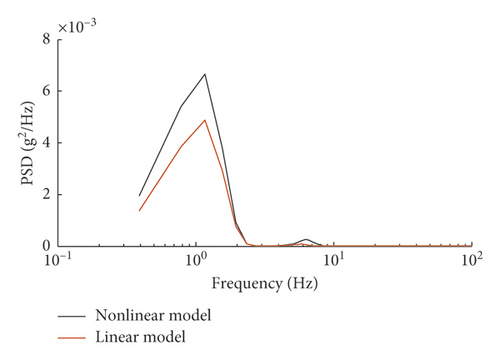
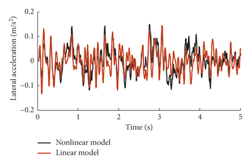
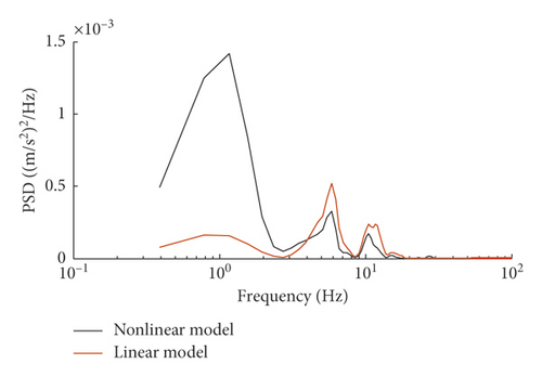
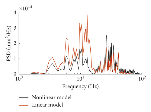
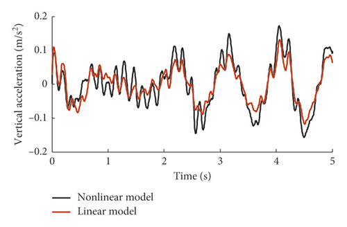
Figures 3 and 4 show the comparisons on the lateral and vertical accelerations of the car body. As seen from these two figures, though there exists unavoidable discrepancy between the models on response amplitudes, the tendency of the time-domain responses of the linear model coincides well with that of the nonlinear model; moreover, the dominant frequencies of the car body accelerations drawn from these two models are almost the same. For the vertical acceleration of the car body, the absolute maximum values are 1.6 m/s2 and 1.41 m/s2; with respect to the nonlinear model and linear model, the dominant frequencies are 1.17 Hz and 6.25 Hz. While for the lateral acceleration, the absolute maximum values of the nonlinear and linear model are 0.145 m/s2 and 0.144 m/s2, respectively; besides, the domain frequencies for these two models are 1.72 Hz, 5.46 Hz, and 10.94 Hz and are similar, but there exists a slight difference in spectral densities inevitably.
Details are in the caption following the image
Comparison of the vertical acceleration of the car body between the linear model and the nonlinear model in the (a) time domain and (b) frequency domain.
Details are in the caption following the image
Comparison of the vertical acceleration of the car body between the linear model and the nonlinear model in the (a) time domain and (b) frequency domain.
Details are in the caption following the image
Comparison of the lateral acceleration of the car body between the linear model and the nonlinear model in the (a) time domain and (b) frequency domain.
Details are in the caption following the image
Comparison of the lateral acceleration of the car body between the linear model and the nonlinear model in the (a) time domain and (b) frequency domain.
Instead of calculating the wheel-rail force using the nonlinear Hertzian contact theory [43]:
F v = K δ 32 / , ()
where K is the Hertz contact coefficient and δ is the wheel-rail relative elastic compression, the wheel-rail vertical force Fv in this paper is obtained by introducing D’Alembert’s principle:
i F i m i a i Δ r i = 0 , ()
where i is an integer indicating a variable; Fi is the total applied force on the i-th particle; mi is the mass of the i-th particle; ai is the acceleration, and Δri is the virtual displacement of the i-th particle; Fvconsists of the rolling force Froll, vertical inertial force Finer, and gravitational force Fgrav, namely, Fv = Froll + Finer + Fgrav.
As an example, the forces acting on the left side of the wheelsets can be written, respectively, as
F roll , i = m c y ¨ c 4 I cz ψ ¨ c 4 l c H cb + H bt + H tw + R w 2 b 0 I cx ϕ c 8 b o + m Gq y ¨ Gq 4 b 0 H tw + R w I Gqx ϕ Gq 4 b 0 1 i + 1 I Gqz ψ ¨ Gq 2 l t H tw + R w 2 b 0 , F roll , i = m c z ¨ c 4 I cy β ¨ c 4 l c + m Gq z ¨ Gq 2 1 i + 1 I Gq , y β ¨ Gq 2 l t + m w , i z ¨ w , i , F grav , i = m w g 2 , ()
where the subscript “i”, i = 1,2,3,4, denotes the ith wheelset; the subscript “Gq” represents the front bogie frame, which is only applicable for i = 1 and 2; when i = 3 or 4, the parameters “mGq,” “ y ¨ Gq ,” “ z ¨ G q ,” “IGq,x,” “ ϕ ¨ Gq ,” “IGq,z,” “ ψ ¨ Gq ,” “IGq,y,” and “ β ¨ Gq ” should be substituted by “mGh,” “ y ¨ Gh ,” “ z ¨ Gh ,” “IGh,x,” “ ϕ ¨ Gh ,” “IGh,z,” “ ψ ¨ Gh ,” “IGh,y,” and “ β ¨ Gh ,” respectively, in which the subscript “Gh” represents the rear bogie frame; b0 denotes the half of the lateral distance between the two wheel-rail contact point at the initial condition; Rwis the nominal rolling radius of the wheel; and Htw is the vertical distance between the centroid of bogie frame and the central line of the wheelset.

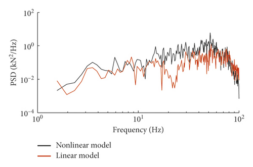
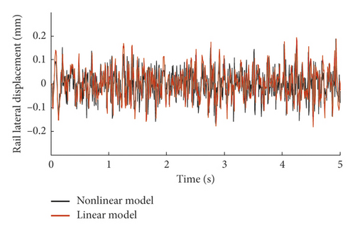
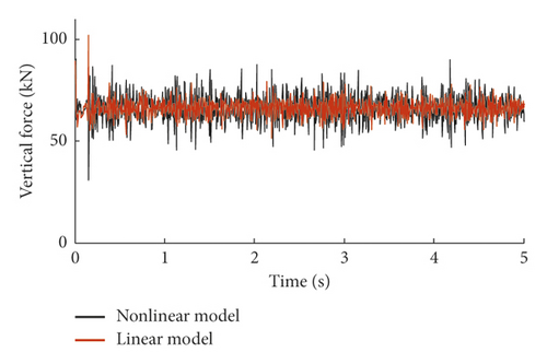
Figure 5 illustrates the discrepancy of the wheel-rail vertical force between the nonlinear model and the linear model due to the implementation of different wheel-rail coupling models. As observed from Figure 4, there is a significant correlation between the results of these two models; see for instance, the sections possessing violent wheel-rail interactions are almost the same, but the forces derived by the nonlinear model are locally larger than those of the linear model, especially at high frequency ranges shown in Figure 5(b), because the time interval of integration of the nonlinear model should be greatly smaller than the linear model for guaranteeing the stability of time integration. Moreover, Figure 6 shows the dynamic responses of the rail lateral displacement at both time and frequency domains, from which one can observe that the results of these two models coincide well with each other. The linear model has accurately characterized the dominant frequencies of rail lateral displacement in the whole frequency range of 1–200 Hz though there are differences in spectral values.
Details are in the caption following the image
Comparison of the wheel-rail vertical force between the linear model and the nonlinear model in the (a) time domain and (b) frequency domain.
Details are in the caption following the image
Comparison of the wheel-rail vertical force between the linear model and the nonlinear model in the (a) time domain and (b) frequency domain.
Details are in the caption following the image
Comparison of rail lateral displacement between the linear model and the nonlinear model in the (a) time domain and (b) frequency domain.
Details are in the caption following the image
Comparison of rail lateral displacement between the linear model and the nonlinear model in the (a) time domain and (b) frequency domain.

In the numerical calculation, if the railway vehicle moves on the track for one second, the computation time for the linear model is 15 sec, while for the nonlinear model, it is 156 sec in MATLAB®, and thus the computational efficiency has been significantly improved.

4.2. Random Vibrations concerning Randomness of Creep Coefficients

Creep coefficient possesses key influence on wheel-rail tangential interactions. Through numerical investigations, it is noticed that the lateral creep coefficient CY in the linearized model will majorly determine the vehicle-track lateral dynamics under irregular excitations. Undoubtedly, the creep coefficients are time-dependent and show randomicity. For obtaining more complete results, there is a necessity to treat the model as an ergodic dynamical system where the most influential parameters, e.g., creep coefficient, should be considered with an ergodicity.

In this study, in order to ensure the reliability of dynamic assessment of a linear model, further work on random vibration analysis will be probed into, where the detailed procedures can be illustrated as follows:
  • (1)

    To reveal the full amplitude and probability characteristics of the creep coefficients, the track irregularity probabilistic model [42] and the nonlinear vehicle-track coupled model [11] are applied to characterize the probability density function (PDF) of CY.

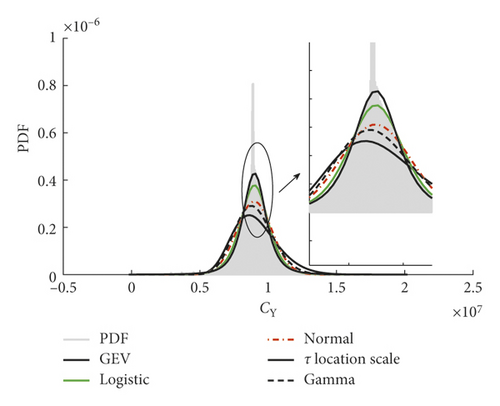
As an example, Figure 7 plots the PDF fitting results of lateral creep coefficient, from which it is found out that the τ location-scale distribution can be properly used to reflect the probability property of the creep coefficients, where τ location-scale distribution can be expressed by
f x = Γ υ + 12 / υ π Γ υ / 2 1 + x μ / σ 2 / υ υ + 1 / 2 , ()
where Γ(⋅) is the gamma function and μ, σ, and υ denote the location, scale, and shape parameter, respectively.
  • (2)

    Since the PDF of CY denoted by pCy is obtained in the above step, the methods for random parameters selection presented in Ref. [5] can be implemented to get the represented random field of CY, that is, ΩCy.

  • (3)

    Set H(·) as the operator of vehicle-track interaction model and loading ΩCy and track irregularity vector TIrre into H(·), the random vibration of vehicle-track systems Rindi can be calculated out consequently, that is,
R indi = H Ω Cy T irre , ()
where the subscript “indi” denotes the dynamic indices of vehicle-track systems.
Details are in the caption following the image
PDF fitting for lateral creep coefficient (GEV, generalized extreme value).
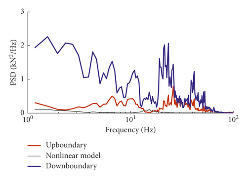
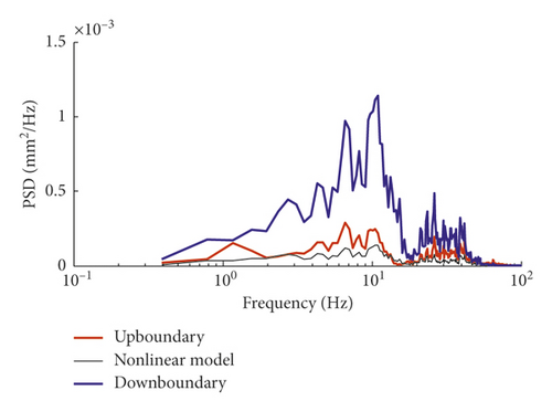
Figure 8 plots the up and down boundary of power spectral density (PSD), denoted by Pu and Pd, respectively, of rail lateral displacement and wheel-rail lateral force, respectively, within which the confidence probability is 99%, that is,
P r u d ω = P u x P d x f P i ndi x ; ω d x = 0.99 , ()
where Pr(·) denotes the probability function; ω is the frequency; f P indi x ; ω is the PDF of spectral densities against specific frequency ω; and x is the spectral density. The red lines are the PSD results of the nonlinear model.
Details are in the caption following the image
The up- and downboundary PSDs of the linear model and the PSD of the nonlinear model. (a) Rail lateral displacement. (b) Wheel-rail lateral force.
Details are in the caption following the image
The up- and downboundary PSDs of the linear model and the PSD of the nonlinear model. (a) Rail lateral displacement. (b) Wheel-rail lateral force.
It can be observed from Figure 8 that the boundary PSDs derived by the linear model can properly envelop the results of the nonlinear model, based on the mathematical relationship between spectral density and time-domain amplitude, that is,
A = 1 π ω i 1 ω i P ω d ω . ()

It is obvious that time-domain responses of the linear model will inevitably envelop those of the nonlinear model. Therefore, with an implementation of the random vibration analysis, the results derived by the linear model can be provided as a reference to guarantee the safety margin of the vehicle-track dynamic behaviours.

However, it should be noted that though the linear model is capable of characterizing the characteristic frequencies of dynamic indices, the chosen of the creep coefficient will exert significant influence on the response amplitude; moreover, the responses of wheel-rail lateral force at low frequency of 10 Hz below will increase violently, which should be treated as one of the deficiencies of the linear model with an emphasis. It is therefore a rather important work to choose the creep coefficient optimally.

5. Conclusions

In this study, the modelling framework for vehicle-track interactions is proposed with linearized wheel-rail contacts/creepages. Key steps for modelling the vehicle-track interactions lie in the establishment of the coupling matrices between subsystems of a vehicle and the tracks and the WRI elements. The correctness and the higher efficiency of the proposed linear model have been presented in the numerical examples; besides, the following conclusions can be drawn accordingly:
  • (1)

    The linearized model can give approachable results to the nonlinear model regarding the response amplitudes and the main dominant frequencies characterized by these two models are also similar. However, there exist obvious differences in frequency spectrum amplitude.

  • (2)

    This presented model possesses higher computational stability due to the linearization. However, this linearization might lead to acceptable deviations in engineering practice comparing to the nonlinear model.

  • (3)

    In this dynamic condition, the system responses at low frequency range of 0–16.5 Hz will be significantly enlarged by the increase of the lateral creep coefficient.

  • (4)

    This current work shows limitations for dynamics problems related to transients, discrete joints, derailment, etc.

Conflicts of Interest

The authors declare that there are no conflicts of interest regarding the publication of this article.

Acknowledgments

This work was supported by the National Key Research and Development Program of China (grant no. 2016YFB120050).

    Appendix

    A. Matrix Formulation for Vehicle System

    Θ sz 1 = z c ϕ c β c z Gq ϕ Gq , K sz 1 Θ sz 1 , Θ sz 1 = k sz N sz 11 , T N sz 11 , + N sz 12 , T N sz 12 , , Θ sz 2 = z c ϕ c β c z Gh ϕ Gh , K sz 2 Θ sz 2 , Θ sz 2 = k sz N sz 21 , T N sz 21 , + N sz 22 , T N sz 22 , , Θ sy 1 = y c ϕ c ψ c y Gq ϕ Gq , K sy 1 Θ sy 1 , Θ sy 1 = 2 k sy N sy 1 T N sy 1 , Θ sy 2 = y c ϕ c ψ c y Gh ϕ Gh , K sy 2 Θ sy 2 , Θ sy 2 = 2 k sy N sy 2 T N sy 2 , Θ sx 1 = ψ c ψ Gq β c β Gq , K sx 1 Θ sx 1 , Θ sx 1 = k sx N sx 11 , T N sx 11 , + N sx 12 , T N sx 12 , , Θ sx 2 = ψ c ψ Gh β c β Gh , K sx 2 Θ sx 2 , Θ sx 2 = k sx N sx 21 , T N sx 21 , + N sx 22 , T N sx 22 , , N sz 11 , = 1 d s l c 1 d s , N sz 12 , = 1 d s l c 1 d s , N sz 21 , = 1 d s l c 1 d s , N sz 22 , = 1 d s l c 1 d s , N sy 1 = 1 H cb l c 1 H bt , N sy 2 = 1 H cb l c 1 H bt , N sx 11 , = d s d s H cb H bt , N sx 12 , = d s d s H cb H bt , N s x 21 , = d s d s H cb H bt , N sx 22 , = d s d s H cb H bt , ()
    where ds is the half of the lateral distance of the secondary suspension, lc is the semilongitudinal distance between bogies, Hbt is the vertical distance between the bottom plane of the secondary suspension and the center of mass of the bogie, and Hcb is the vertical distance between centroids of car body and side bogie.

    B. Matrix Formulation for Vehicle-WRT Coupled System

    K vr , z = K vr, z 1 Θ vr, z 1 , Θ vr, z 1 + K vr , z 2 Θ vr , z 2 , Θ vr , z 2 + K vr, z 3 Θ vr, z 3 , Θ vr, z 3 + K vr , z 4 Θ vr, z 4 , Θ vr , z 4 , K vr , y = K vr, y 1 Θ vr, y 1 , Θ vr, y 1 + K vr , y 2 Θ vr , y 2 , Θ vr , y 2 + K vr, y 3 Θ vr, y 3 , Θ vr, y 3 + K vr , y 4 Θ vr , y 4 , Θ vr , y 4 , K vr , x = K vr, x 1 Θ vr, x 1 , Θ vr, x 1 + K vr , x 2 Θ vr , x 2 , Θ vr , x 2 + K vr, x 3 Θ vr, x 3 , Θ vr, x 3 + K vr , x 4 Θ vr , x 4 , Θ vr , x 4 , Θ vr, z 1 = z Gq L v , 1 L z , 1 R v , 1 R z , 1 ϕ Gq β Gq , Θ vr, z 2 = z Gq L v , 2 L z , 2 R v , 2 R z , 2 ϕ Gq β Gq , Θ vr, z 3 = z Gh L v , 3 L z , 3 R v , 3 R z , 3 ϕ Gh β Gh , Θ vr, z 4 = z Gh L v , 4 L z , 4 R v , 4 R z , 4 ϕ Gh β Gh , Θ vr, y 1 = y Gq y w 1 ϕ Gq ψ Gq , Θ vr, y 2 = y Gq y w 2 ϕ Gq ψ Gq , Θ vr, y 3 = y Gh y w 3 ϕ Gh ψ Gh , Θ vr, y 4 = y Gh y w 4 ϕ Gh ψ Gh , Θ vr, x 1 = x Gq x w 1 ψ Gq ψ w 1 ϕ Gq , Θ vr, x 2 = x Gq x w 2 ψ Gq ψ w 2 ϕ Gq , Θ vr, x 3 = x Gh x w 3 ψ Gh ψ w 3 ϕ Gh , Θ vr, x 4 = x Gh x w 4 ψ Gh ψ w 4 ϕ Gh , K vr, z 1 Θ vr, z 1 , Θ vr, z 1 = k pz N vr , z 11 , T N vr , z 11 , + N vr , z 12 , T N vr , z 12 , , N vr , z 11 , = 1 1 2 1 2 1 2 1 2 d w l t , N vr , z 12 , = 1 1 2 1 2 1 2 1 2 d w l t , K vr,z 2 Θ vr,z 2 , Θ vr,z 2 = k pz N vr , z 21 , T N vr , z 21 , + N vr , z 22 , T N vr , z 22 , , N vr , z 21 , = 1 1 2 1 2 1 2 1 2 d w l t , N vr , z 22 , = 1 1 2 1 2 1 2 1 2 d w l t , K vr,z 3 Θ vr,z 3 , Θ vr,z 3 = k pz N vr , z 3,1 T N vr , z 3,1 + N vr , z 3,2 T N vr , z 3,2 , N vr , z 3,1 = N vr , z 11 , , N vr , z 3,2 = N vr , z 12 , , K vr,z 4 Θ vr,z 4 , Θ vr,z 4 = k pz N vr , z 4,1 T N v r , z 4,1 + N vr , z 4,2 T N vr , z 4,2 , N vr , z 4,1 = N vr , z 21 , , N vr , z 4,2 = N vr , z 22 , , K vr, y 1 Θ vr, y 1 , Θ vr, y 1 = 2 k py N vr , y 1 T N v r , y 1 , N vr , y 1 = 1 1 H t w l t , K vr, y 2 Θ vr, y 2 , Θ vr, y 2 = 2 k py N vr , y 2 T N vr , y 2 , N vr , y 2 = 1 1 H tw l t , K vr, y 3 Θ vr, y 3 , Θ vr, y 3 = 2 k py N vr , y 3 T N vr , y 3 , N vr , y 3 = N vr , y 1 , K vr, y 4 Θ vr, y 4 , Θ vr, y 4 = 2 k py N vr , y 4 T N vr , y 4 , N vr , y 4 = N vr , y 2 , K vr, x 1 Θ vr,x 1 , Θ vr,x 1 = k px N vr , x 11 , T N vr , x 11 , + N vr , x 12 , T N vr , x 12 , , N vr , x 11 , = 1 1 d w d w H t w , N vr , x 12 , = 1 1 d w d w H t w , K vr, x 2 Θ vr, x 2 , Θ vr, x 2 = k px N vr , x 21 , T N vr , x 21 , + N vr , x 22 , T N vr , x 22 , , N vr , x 21 , = N vr , x 11 , , N vr , x 22 , = N vr , x 12 , , K vr, x 3 Θ vr, x 3 , Θ vr, x 3 = k px N vr , x 3,1 T N v r , x 3,1 + N v r , x 3,2 T N vr , x 3,2 , N vr , x 3,1 = N vr , x 11 , , N vr , x 3,2 = N vr , x 12 , , K vr, x 4 Θ vr, x 4 , Θ vr, x 4 = k px N vr , x 4,1 T N vr , x 4,1 + N vr , x 4,2 T N vr , x 4,2 , N vr , x 4,1 = N vr , x 11 , , N vr , x 4,2 = N vr , x 12 , , ()
    where dw is the half of the lateral distance of the primary suspension, lw is the semilongitudinal distance between two wheelsets in a bogie frame, Htw is the vertical distance between the centroid of side frame and the center line of wheelset, and kpz, kpy, and kpx represent the vertical, lateral, and longitudinal stiffness of the primary suspension.

    Data Availability

    The data we used in this paper for calculation, analysis, and formula derivation are included in this paper or can be found in the references listed in this paper.

      The full text of this article hosted at iucr.org is unavailable due to technical difficulties.