The approximate analytical solution of the fractional Cahn-Hilliard and Gardner equations has been acquired successfully via residual power series method (RPSM). The approximate solutions obtained by RPSM are compared with the exact solutions as well as the solutions obtained by homotopy perturbation method (HPM) and q-homotopy analysis method (q-HAM). Numerical results are known through different graphs and tables. The fractional derivatives are described in the Caputo sense. The results light the power, efficiency, simplicity, and reliability of the proposed method.

1. Introduction

Fractional differential equations (FDEs) have found applications in many problems in physics and engineering [1, 2]. Since most of the nonlinear FDEs cannot be solved exactly, approximate and numerical methods must be used. Some of the recent analytical methods for solving nonlinear problems include the Adomian decomposition method [3, 4], variational iteration method [5], homotopy perturbation method [6, 7], homotopy analysis method [8, 9], spectral collocation method [10], the tanh-coth method [11], exp-function method [12], Mittag-Leffler function method [13], differential quadrature method [14], and reproducing kernel Hilbert space method [15, 16].

The Gardner equation [17] (combined KdV-mKdV equation) is a useful model for the description of internal solitary waves in shallow water,

()

Those two models will be classified as positive Gardner equation and negative Gardner equation depending on the sign of the cubic nonlinear term [18, 19]. Gardner equation is widely used in various branches of physics, such as plasma physics, fluid physics, and quantum field theory [20, 21]. It also describes a variety of wave phenomena in plasma and solid state [22, 23].

The Cahn-Hilliard equation [24] is one type of partial differential equations (PDEs) and was first introduced in 1958 as a model for process of phase separation of a binary alloy under the critical temperature [25],

()

This equation is related to a number of interesting physical phenomena like the spinodal decomposition, phase separation, and phase ordering dynamics. On the other hand it becomes important in material sciences [26, 27].

The aim of this paper is to study the time-fractional Gardner equation [28–30] and time-fractional Cahn-Hilliard equation [31–37] of this form,

()

where 0 < α ≤ 1, −∞ < x < ∞, and 0 ≤ t < R. Numerous methods have been used to solve this equations, for example, q-Homotopy analysis method [28], the new version of F-expansion method [29], reduced differential transform method [30], the generalized tanh-coth method [38], the generalized Kudryashov method [39], extended fractional Riccati expansion method [31], subequation method [32], homotopy analysis method [33], the Adomian decomposition method [34], improved

expansion method [35], homotopy perturbation method [36], and variational iteration method [37]. We solve Cahn-Hilliard equation and Gardner equation by RPSM.

The RPSM was first devised in 2013 by the Jordanian mathematician Omar Abu Arqub as an efficient method for determining values of coefficients of the power series solution for first and the second-order fuzzy differential equations [40]. The RPSM is an effective and easy to construct power series solution for strongly linear and nonlinear equations without linearization, perturbation, or discretization. In the last few years, the RPSM has been applied to solve a growing number of nonlinear ordinary and PDEs of different types, classifications, and orders. It has been successfully applied in the numerical solution of the generalized Lane-Emden equation [41], which is a highly nonlinear singular differential equation, in the numerical solution of higher-order regular differential equations [42], in approximate solution of the nonlinear fractional KdV-Burgers equation [43], in construct and predict the solitary pattern solutions for nonlinear time-fractional dispersive PDEs [44], and in predicting and representing the multiplicity of solutions to boundary value problems of fractional order [45]. The RPSM distinguishes itself from various other analytical and numerical methods in several important aspects [46]. Firstly, the RPSM does not need to compare the coefficients of the corresponding terms and a recursion relation is not required. Secondly, the RPSM provides a simple way to ensure the convergence of the series solution by minimizing the related residual error. Thirdly, the RPSM is not affected by computational rounding errors and does not require large computer memory and time. Fourthly, the RPSM does not require any converting while switching from the low-order to the higher-order and from simple linearity to complex nonlinearity; as a result, the method can be applied directly to the given problem by choosing an appropriate initial guess approximation.

2. Fundamental Concepts

Definition 1 (see [43].)The Caputo time-fractional derivatives of order α > 0 of u(x, t) is defined as

()

Definition 2 (see [47], [48].)A power series representation of the form

()

where 0 ≤ n − 1 < α ≤ n, n ∈ N and t ≥ t₀ is called fractional power series about t₀.

Theorem 3 (see [47], [48].)Suppose that f has a fractional power series representation at t₀ of the form

()

If D^nαf(t) are continuous on (t₀, t₀ + R), n = 0,1, 2,3, …, then coefficients C_n will take the form

()

Definition 4 (see [43].)A power series representation of the form

()

is called a multiple fractional power series about t = t₀.

Theorem 5 (see [43], [44].)Suppose that u(x, t) has a multiple fractional Power series representation at t₀ of the form

()

are continuous on I × (t₀, t₀ + R), n = 0,1, 2,3, …, then coefficients f_n(x) will take the form

()

Corollary 6 (see [44].)Suppose that u(x, y, t) has a multiple fractional Power series representation at t₀ of the form

()

are continuous on I₁ × I₂ × (t₀, t₀ + R), n = 0,1, 2,3, …, then f_n(x, y) will take the form

()

3. Basic Idea of RPSM

To give the approximate solution of nonlinear fractional order differential equations by means of the RPSM, we consider a general nonlinear fractional differential equation:

()

where N(u) is nonlinear term and R(u) is a linear term. Subject to the initial condition

()

The RPSM proposes the solution for (14) as a fractional power series about the initial point t = 0,

()

Next we let u_k(x, t) denote the kth truncated series of u(x, t),

()

The 0th RPS approximate solution of u(x, t) is

()

Equation (17) can be written as

()

We define the residual function for (14)

()

Therefore, the kth residual function Res_u,k is

()

As in [40, 41], since the fractional derivative of a constant in the Caputo sense is zero and the fractional derivatives of Res(x, t) and Res_k(x, t) are matching at t = 0 for each n = 0,1, 2, …., k.; that is, , n = 0,1, 2, …., k.

To determine f₁(x), f₂(x), f₃(x), … we consider k = 1,2, 3.. in (19) and substitute it into (21), applying the fractional derivative

in both sides, k = 1, 2, 3, …, and finally we solve

()

4. Applications

To illustrate the basic idea of RPSM, we consider the following two time-fractional Gardner and Cahn-Hilliard equations.

4.1. Time-Fractional Gardner Equation

Consider the time-fractional homogeneous Gardner equation

()

Subject to the initial Condition

()

The exact solution when ε = 1, α = 1 is

()

We define the residual function for (23) as

()

therefore, for the kth residual function Res_u,k(x, t),

()

To determine f₁(x), we consider (k = 1) in (27)

()

But from (19) at k = 1,

()

Now depending on the result of (22) In the case of k=1, we have

()

To determine f₂(x), we consider (k = 2) in (27)

()

But from (19) at k = 2,

()

Applying

on both sides and solving the equation

, then we get

()

The solution in series form is given by

()

4.2. Time-Fractional Cahn-Hilliard Equation

Consider the time-fractional Cahn-Hilliard equation

()

Subject to the initial condition

()

The exact solution when α = 1 is

()

We define the residual function for (39) as

()

therefore, for the kth residual function Res_u,k(x, t),

()

To determine f₁(x), we consider (k = 1) in (43)

()

From (19) at k = 1,

()

If we put Res_u,1(x, 0) = 0, then

()

Similarity, to determine f₂(x), we substitute

()

into (43) where k = 2,

()

Solving the equation

, we find that

()

To determine f₃(x), we substitute

()

into (43) where k=3,

()

Applying

on both sides and then solving the equation

, we get

()

The solution in series form is given by

()

5. Numerical Results

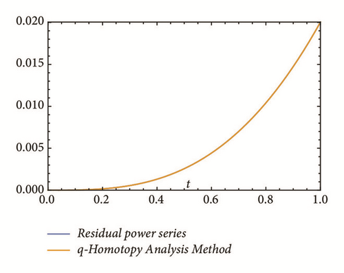
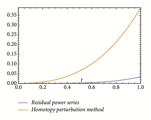
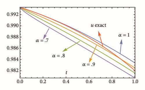
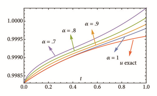
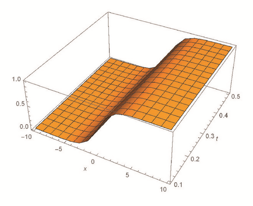
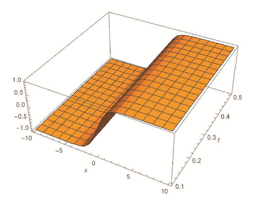
This section deals with the approximate analytical solutions obtained by RPSM for Gardner and Cahn-Hilliard equations. In classical case(α → 1), Figure 1 and Tables 1 and 2 describe the comparison between RPSM with q-HAM [28] and HPM [36]. In fractional case, Figures 2, 3, and 4 describe the geometrical behavior of the solutions obtained by RPSM for different fractional value α of the two equations.

Table 1. The absolute errors |u_exact − u₃| for Gardner equation when t = .2, ε = 1, α → 1.

x	\|u_exact − u_RPS\|	\|u_exact − u_qHAM\|
.1	166.002 × 10⁻⁶	166.002 × 10⁻⁶
.2	162.707 × 10⁻⁶	162.707 × 10⁻⁶
.3	156.257 × 10⁻⁶	156.257 × 10⁻⁶
.4	146.917 × 10⁻⁶	146.917 × 10⁻⁶
.5	135.064 × 10⁻⁶	135.064 × 10⁻⁶

Table 2. The absolute errors |u_exact − u₄| for Cahn-Hilliard when t = .2, α → 1.

x	\|u_exact − u_RPS\|	\|u_exact − u_HPM\|
.1	25.5541 × 10⁻⁶	4.68338 × 10⁻³
.2	41.5291 × 10⁻⁶	7.28902 × 10⁻³
.3	54.2246 × 10⁻⁶	9.6162 × 10⁻³
.4	62.8898 × 10⁻⁶	11.5931 × 10⁻³
.5	67.2637 × 10⁻⁶	13.174 × 10⁻³

Details are in the caption following the image — **Figure 1 (a)**
Open in figure viewer PowerPoint

(a) Absolute errors of fractional Gardner equation, at x = 2, ε = 1. (b) Absolute errors of fractional Chan-Hilliard equation at x = 2.

6. Conclusions

This work has used the RPSM for finding the solution of the time-fractional Gardner and Cahn-Hilliard equations. A very good agreement between the results obtained by the RPSM and q-HAM [28] was observed in Figure 1(a) and Table 1. Figure 1(b) and Table 2 indicate that the mentioned method achieves a higher level of accuracy than HPM [36]. Consequently, the work emphasized that the method introduces a significant improvement in this field over existing techniques.

Conflicts of Interest

The authors declare that they have no conflicts of interest.

Open Research

Data Availability

[1] The [approximate solution obtained by q-homotopy analysis method] data used to support the findings of this study have been deposited in the [article] repository ([doi.org/10.1016/j.asej.2014.03.014]) [28]. [2] The [approximate solution obtained by homotopy perturbation method] data used to support the findings of this study have been deposited in the [article] repository ([doi.org/10.1080/10288457.2013.867627]) [36].

References

1 Debnath L., Recent applications of fractional calculus to science and engineering, International Journal of Mathematics and Mathematical Sciences. (2003) no. 54, 3413–3442, https://doi.org/10.1155/S0161171203301486, MR2025566, Zbl1036.26004, 2-s2.0-17844372193.
10.1155/S0161171203301486
Google Scholar
2 Rahimy M., Applications of fractional differential equations, Applied Mathematical Sciences. (2010) 4, no. 49-52, 2453–2461, MR2726272, Zbl1220.34005, 2-s2.0-78149483277.
Google Scholar
3 Arafa A. A. and Rida S. Z., Numerical solutions for some generalized coupled nonlinear evolution equations, Mathematical and Computer Modelling. (2012) 56, no. 11-12, 268–277, https://doi.org/10.1016/j.mcm.2011.12.046, MR2974546, Zbl1255.65179.
10.1016/j.mcm.2011.12.046
Google Scholar
4 Arafa A. A., Series solutions of time-fractional host-parasitoid systems, Journal of Statistical Physics. (2011) 145, no. 5, 1357–1367, https://doi.org/10.1007/s10955-011-0339-z, MR2863738, Zbl1375.92044, 2-s2.0-82255174920.
10.1007/s10955-011-0339-z
Web of Science® Google Scholar
5 Sweilam N. H., Khader M. M., and Al-Bar R. F., Numerical studies for a multi-order fractional differential equation, Physics Letters A. (2007) 371, no. 1-2, 26–33, https://doi.org/10.1016/j.physleta.2007.06.016, MR2419274, Zbl1209.65116.
10.1016/j.physleta.2007.06.016
CAS Web of Science® Google Scholar
6 Golbabai A. and Sayevand K., Fractional calculus- a new approach to the analysis of generalized fourth-order diffusion-wave equations, Computers & Mathematics with Applications. An International Journal. (2011) 61, no. 8, 2227–2231, https://doi.org/10.1016/j.camwa.2010.09.022, MR2785590.
10.1016/j.camwa.2010.09.022
Web of Science® Google Scholar
7 Gepreel K. A., The homotopy perturbation method applied to the nonlinear fractional Kolmogorov-Petrovskii-PISkunov equations, Applied Mathematics Letters. (2011) 24, no. 8, 1428–1434, https://doi.org/10.1016/j.aml.2011.03.025, MR2793646, Zbl1219.35347.
10.1016/j.aml.2011.03.025
Web of Science® Google Scholar
8 Arafa A. A., Rida S. Z., and Mohamed H., Approximate analytical solutions of Schnakenberg systems by homotopy analysis method, Applied Mathematical Modelling: Simulation and Computation for Engineering and Environmental Systems. (2012) 36, no. 10, 4789–4796, https://doi.org/10.1016/j.apm.2011.12.014, MR2930371, Zbl1252.65173.
10.1016/j.apm.2011.12.014
Google Scholar
9 Arafa A. A., Rida S. Z., and Khalil M., The effect of anti-viral drug treatment of human immunodeficiency virus type 1 ({HIV}-1) described by a fractional order model, Applied Mathematical Modelling: Simulation and Computation for Engineering and Environmental Systems. (2013) 37, no. 4, 2189–2196, https://doi.org/10.1016/j.apm.2012.05.002, MR3002310, Zbl1349.92135.
10.1016/j.apm.2012.05.002
Google Scholar
10 Javidi M., A numerical solution of the generalized Burgers-Huxley equation by spectral collocation method, Applied Mathematics and Computation. (2006) 178, no. 2, 338–344, https://doi.org/10.1016/j.amc.2005.11.051, MR2248493, Zbl1100.65081, 2-s2.0-33746228097.
10.1016/j.amc.2005.11.051
Web of Science® Google Scholar
11 Wazwaz A.-M., Analytic study on Burgers, Fisher, Huxley equations and combined forms of these equations, Applied Mathematics and Computation. (2008) 195, no. 2, 754–761, https://doi.org/10.1016/j.amc.2007.05.020, MR2381254, Zbl1132.65098, 2-s2.0-37349105607.
10.1016/j.amc.2007.05.020
Web of Science® Google Scholar
12 Zhou X.-W., Exp-function method for solving Huxley equation, Mathematical Problems in Engineering. (2008) Art. ID 538489, 7, https://doi.org/10.1155/2008/538489, MR2402979, Zbl1151.92007.
10.1155/2008/538489
Web of Science® Google Scholar
13 Arafa A. A., Rida S. Z., Mohammadein A. A., and Ali H. M., Solving nonlinear fractional differential equation by generalized Mittag-Leffler function method, Communications in Theoretical Physics. (2013) 59, no. 6, 661–663, https://doi.org/10.1088/0253-6102/59/6/01, MR3155428, 2-s2.0-84880536792.
10.1088/0253-6102/59/6/01
Web of Science® Google Scholar
14 Sari M. and Gürarslan G., Numerical solutions of the generalized Burgers-Huxley equation by a differential quadrature method, Mathematical Problems in Engineering. (2009) Art. ID 370765, 11, https://doi.org/10.1155/2009/370765, MR2491525.
10.1155/2009/370765
Web of Science® Google Scholar
15 Abu Arqub O., An iterative method for solving fourth-order boundary value problems of mixed type integro-differential equations, Journal of Computational Analysis and Applications. (2015) 18, no. 5, 857–874, MR3308505, Zbl1329.65176, 2-s2.0-84985874149.
Web of Science® Google Scholar
16 Abu Arqub O., Fitted reproducing kernel Hilbert space method for the solutions of some certain classes of time-fractional partial differential equations subject to initial and Neumann boundary conditions, Computers & Mathematics with Applications. (2017) 73, no. 6, 1243–1261, https://doi.org/10.1016/j.camwa.2016.11.032.
10.1016/j.camwa.2016.11.032
Web of Science® Google Scholar
17 Wazwaz A.-M., Solitons and singular solitons for the Gardner-{KP} equation, Applied Mathematics and Computation. (2008) 204, no. 1, 162–169, https://doi.org/10.1016/j.amc.2008.06.011, MR2458351, Zbl1159.35432, 2-s2.0-52049114674.
10.1016/j.amc.2008.06.011
Web of Science® Google Scholar
18 Gardner C. S., Greene J. M., Kruskal M. D., and Miura R. M., Method for solving the Korteweg-deVries equation, Physical Review Letters. (1967) 19, no. 19, 1095–1097, 2-s2.0-36049057587, https://doi.org/10.1103/PhysRevLett.19.1095.
10.1103/PhysRevLett.19.1095
CAS Web of Science® Google Scholar
19 Wazwaz A.-M., New solitons and kink solutions for the Gardner equation, Communications in Nonlinear Science and Numerical Simulation. (2007) 12, no. 8, 1395–1404, https://doi.org/10.1016/j.cnsns.2005.11.007, MR2332640, Zbl1118.35352, 2-s2.0-34249735366.
10.1016/j.cnsns.2005.11.007
Web of Science® Google Scholar
20 Fu Z., Liu S., and Liu S., New kinds of solutions to Gardner equation, Chaos, Solitons & Fractals. (2004) 20, no. 2, 301–309, https://doi.org/10.1016/S0960-0779(03)00383-7, MR2025581, Zbl1046.35097, 2-s2.0-0142166467.
10.1016/S0960-0779(03)00383-7
Web of Science® Google Scholar
21 Xu G.-q., Li Z.-b., and Liu Y.-p., Exact solutions to a large class of nonlinear evolution equations, Chinese Journal of Physics. (2003) 41, no. 3, 232–241, MR2010807, 2-s2.0-0043071570.
Web of Science® Google Scholar
22 Baldwin D., Göktas Ü., Hereman W., Hong L., Martino R. S., and Miller J. C., Symbolic computation of exact solutions expressible in hyperbolic and elliptic functions for nonlinear PDEs, Journal of Symbolic Computation. (2004) 37, no. 6, 669–705, https://doi.org/10.1016/j.jsc.2003.09.004, MR2095366.
10.1016/j.jsc.2003.09.004
Web of Science® Google Scholar
23 Hereman W. and Nuseir A., Symbolic methods to construct exact solutions of nonlinear partial differential equations, Mathematics and Computers in Simulation. (1997) 43, no. 1, 13–27, https://doi.org/10.1016/S0378-4754(96)00053-5, MR1438817, Zbl0866.65063, 2-s2.0-0030829213.
10.1016/S0378-4754(96)00053-5
Web of Science® Google Scholar
24 Ugurlu Y. and Kaya D. g., Solutions of the Cahn-Hilliard equation, Computers & Mathematics with Applications. An International Journal. (2008) 56, no. 12, 3038–3045, https://doi.org/10.1016/j.camwa.2008.07.007, MR2474558.
10.1016/j.camwa.2008.07.007
Web of Science® Google Scholar
25 Cahn J. W. and Hilliard J. E., Free energy of a nonuniform system. I. Interfacial free energy, The Journal of Chemical Physics. (1958) 28, no. 2, 258–267, 2-s2.0-33746012315, https://doi.org/10.1063/1.1744102.
10.1063/1.1744102
CAS Web of Science® Google Scholar
26 Choo S. M., Chung S. K., and Lee Y. J., A conservative difference scheme for the viscous Cahn-Hilliard equation with a nonconstant gradient energy coefficient, Applied Numerical Mathematics. (2004) 51, no. 2-3, 207–219, https://doi.org/10.1016/j.apnum.2004.02.006, MR2091400, Zbl1112.65078.
10.1016/j.apnum.2004.02.006
Web of Science® Google Scholar
27 Gurtin M. E., Generalized Ginzburg-Landau and Cahn-Hilliard equations based on a microforce balance, Physica D: Nonlinear Phenomena. (1996) 92, no. 3-4, 178–192, https://doi.org/10.1016/0167-2789(95)00173-5, MR1387065, Zbl0885.35121.
10.1016/0167-2789(95)00173-5
CAS Web of Science® Google Scholar
28 Iyiola O. S. and Olayinka O. G., Analytical solutions of time-fractional models for homogeneous Gardner equation and non-homogeneous differential equations, Ain Shams Engineering Journal. (2014) 5, no. 3, 999–1004, 2-s2.0-84906327174, https://doi.org/10.1016/j.asej.2014.03.014.
10.1016/j.asej.2014.03.014
Google Scholar
29 Pandir Y. and Duzgun H. H., New Exact Solutions of Time Fractional Gardner Equation by Using New Version of F-Expansion Method, Communications in Theoretical Physics. (2017) 67, no. 1, 9–14, 2-s2.0-85012881535, https://doi.org/10.1088/0253-6102/67/1/9, Zbl1357.35287.
10.1088/0253-6102/67/1/9
Web of Science® Google Scholar
30 Ahmad J. and Mohyud-Din S. T., An efficient algorithm for some highly nonlinear fractional PDEs in mathematical physics, PLoS ONE. (2014) 9, no. 12, 2-s2.0-84919667877, https://doi.org/10.1371/journal.pone.0109127, e109127.
10.1371/journal.pone.0109127
PubMed Web of Science® Google Scholar
31 Li W., Yang H., and He B., Exact solutions of fractional Burgers and Cahn-Hilliard equations using extended fractional Riccati expansion method, Mathematical Problems in Engineering. (2014) Art. ID 104069, 9, https://doi.org/10.1155/2014/104069, MR3224383.
10.1155/2014/104069
Google Scholar
32 Jafari H., Tajadodi H., Kadkhoda N., and Baleanu D., Fractional subequation method for Cahn-Hilliard and Klein-Gordon equations, Abstract and Applied Analysis. (2013) 2013, 5, https://doi.org/10.1155/2013/587179, 587179, MR3034884, Zbl06161355.
10.1155/2013/587179
Google Scholar
33 Mohamed M. S. and Mekheimer K. S., Analytical approximate solution for nonlinear space-time fractional Cahn-Hilliard equation, International Electronic Journal of Pure and Applied Mathematics. (2014) 7, no. 4, 145–159, MR3259465, Zbl06774191.
10.12732/iejpam.v7i4.1
Google Scholar
34 Dahmani Z. and Benbachir M., Solutions of the Cahn-Hilliard equation with time- and space-fractional derivatives, International Journal of Nonlinear Science. (2009) 8, no. 1, 19–26, MR2557974, Zbl1179.35263.
Google Scholar
35 Baleanu D., Ugurlu Y., Inc M., and Kilic B., Improved ( G ′ / G ) -Expansion Method for the Time-Fractional Biological Population Model and Cahn–Hilliard Equation, Journal of Computational and Nonlinear Dynamics. (2015) 10, no. 5, https://doi.org/10.1115/1.4029254.
10.1115/1.4029254
Web of Science® Google Scholar
36 Bouhassoun A. and Hamdi Cherif M., Homotopy Perturbation Method For Solving The Fractional Cahn-Hilliard Equation, Journal of Interdisciplinary Mathematics. (2015) 18, no. 5, 513–524, 2-s2.0-84941758387, https://doi.org/10.1080/10288457.2013.867627.
10.1080/10288457.2013.867627
Web of Science® Google Scholar
37 Ahmad J. and Mohyud-Din S. T., An efficient algorithm for nonlinear fractional partial differential equations, Proceedings of the Pakistan Academy of Sciences. (2015) 52, no. 4, 381–388, MR3452511, 2-s2.0-84949222137.
Google Scholar
38 Manafian J. and Lakestani M., A new analytical approach to solve some of the fractional-order partial differential equations, Indian Journal of Physics. (2017) 91, no. 3, 243–258, 2-s2.0-85013335947, https://doi.org/10.1007/s12648-016-0912-z.
10.1007/s12648-016-0912-z
CAS Web of Science® Google Scholar
39 Tuluce Demiray S., Pandir Y., and Bulut H., Generalized Kudryashov method for time-fractional differential equations, Abstract and Applied Analysis. (2014) Art. ID 901540, 13, https://doi.org/10.1155/2014/901540, MR3240569.
10.1155/2014/901540
Google Scholar
40 Abu Arqub O., Series solution of fuzzy differential equations under strongly generalized differentiability, Journal of Advanced Research in Applied Mathematics. (2013) 5, no. 1, 31–52, https://doi.org/10.5373/jaram.1447.051912.
10.5373/jaram.1447.051912
Google Scholar
41 Abu Arqub O., El-Ajou A., Bataineh A. S., and Hashim I., A representation of the exact solution of generalized Lane-Emden equations using a new analytical method, Abstract and Applied Analysis. (2013) Art. ID 378593, 10, MR3073508, Zbl1291.34024.
10.1155/2013/378593
Google Scholar
42 Abu Arqub O., Abo-Hammour Z., Al-Badarneh R., and Momani S., A reliable analytical method for solving higher-order initial value problems, Discrete Dynamics in Nature and Society. (2013) 2013, 12, https://doi.org/10.1155/2013/673829, 673829, MR3145428.
10.1155/2013/673829
Web of Science® Google Scholar
43 El-Ajou A., Abu Arqub O., and Momani S., Approximate analytical solution of the nonlinear fractional KdV-Burgers equation: a new iterative algorithm, Journal of Computational Physics. (2015) 293, 81–95, https://doi.org/10.1016/j.jcp.2014.08.004, MR3342458, Zbl1349.65546, 2-s2.0-84937057969.
10.1016/j.jcp.2014.08.004
Web of Science® Google Scholar
44 Arqub O. A., El-Ajou A., and Momani S., Constructing and predicting solitary pattern solutions for nonlinear time-fractional dispersive partial differential equations, Journal of Computational Physics. (2015) 293, 385–399, https://doi.org/10.1016/j.jcp.2014.09.034, MR3342478, Zbl1349.35394, 2-s2.0-84937057968.
10.1016/j.jcp.2014.09.034
Web of Science® Google Scholar
45 Arqub O. A., El-Ajou A., Zhour Z. A., and Momani S., Multiple solutions of nonlinear boundary value problems of fractional order: A new analytic iterative technique, Entropy. (2014) 16, no. 1, 471–493, 2-s2.0-84893183719, https://doi.org/10.3390/e16010471.
10.3390/e16010471
Web of Science® Google Scholar
46 El-Ajou A., Abu Arqub O., Momani S., Baleanu D., and Alsaedi A., A novel expansion iterative method for solving linear partial differential equations of fractional order, Applied Mathematics and Computation. (2015) 257, 119–133, https://doi.org/10.1016/j.amc.2014.12.121, MR3320653, Zbl1339.65201, 2-s2.0-84925508576.
10.1016/j.amc.2014.12.121
Web of Science® Google Scholar
47 El-Ajou A., Abu Arqub O., Al Zhour Z., and Momani S., New results on fractional power series: theories and applications, Entropy. An International and Interdisciplinary Journal of Entropy and Information Studies. (2013) 15, no. 12, 5305–5323, https://doi.org/10.3390/e15125305, MR3147055, Zbl1337.26010.
10.3390/e15125305
Google Scholar
48 El-Ajou A., Abu Arqub O., and Al-Smadi M., A general form of the generalized Taylor′s formula with some applications, Applied Mathematics and Computation. (2015) 256, 851–859, https://doi.org/10.1016/j.amc.2015.01.034, MR3316113, Zbl1338.40007.
10.1016/j.amc.2015.01.034
Web of Science® Google Scholar

Citing Literature

All articles

Application of Residual Power Series Method to Fractional Coupled Physical Equations Arising in Fluids Flow

Abstract

1. Introduction

2. Fundamental Concepts

3. Basic Idea of RPSM

4. Applications

4.1. Time-Fractional Gardner Equation

4.2. Time-Fractional Cahn-Hilliard Equation

5. Numerical Results

6. Conclusions

Conflicts of Interest

Open Research

Data Availability

References

Citing Literature

Figures

References

Information

About Wiley Online Library

Help & Support

Opportunities

Connect with Wiley

Application of Residual Power Series Method to Fractional Coupled Physical Equations Arising in Fluids Flow

Abstract

1. Introduction

2. Fundamental Concepts

3. Basic Idea of RPSM

4. Applications

4.1. Time-Fractional Gardner Equation

4.2. Time-Fractional Cahn-Hilliard Equation

5. Numerical Results

6. Conclusions

Conflicts of Interest

Open Research

Data Availability

References

Citing Literature

Figures

References

Related

Information