The Probabilities of Trees and Cladograms under Ford’s α-Model
Abstract
Ford’s α-model is one of the most popular random parametric models of bifurcating phylogenetic tree growth, having as specific instances both the uniform and the Yule models. Its general properties have been used to study the behavior of phylogenetic tree shape indices under the probability distribution it defines. But the explicit formulas provided by Ford for the probabilities of unlabeled trees and phylogenetic trees fail in some cases. In this paper we give correct explicit formulas for these probabilities.
1. Introduction
The study of random growth models of rooted phylogenetic trees and the statistical properties of the shapes of the phylogenetic trees they produce was initiated almost one century ago by Yule [1] and it has gained momentum in the last 20 years: see, for instance, [2–8]. The final goal of this line of research is to understand the relationship between the forces that drive evolution and the topological properties of “real-life” phylogenetic trees [3, 9]; see also [10, Chapter 33]. One of the most popular such models is Ford’s α-model for rooted bifurcating phylogenetic trees or cladograms [4]. It consists of a parametric model that generalizes both the uniform model (where new leaves are added equiprobably to any arc, giving rise to the uniform probability distribution on the sets of cladograms with a fixed set of taxa) and Yule’s model (where new leaves are added equiprobably only to pendant arcs, i.e., to arcs ending in leaves) by allocating a possibly different probability (that depends on a parameter α and hence its name, “α-model”) to the addition of the new leaves to pendant arcs or to internal arcs.
When models like Ford’s model are used to contrast topological properties of phylogenetic trees contained in databases like TreeBase (https://treebase.org), only their general properties (moments, asymptotic behavior) are employed. But, in the course of a research where we have needed to compute the probabilities of several specific cladograms under this model [11], we have noticed that the explicit formulas that Ford gives in [4, §3.5] for the probabilities of cladograms and of tree shapes (unlabeled rooted bifurcating trees) are wrong, failing for some trees with n⩾8 leaves; see Propositions 29 and 32 in [4], with the definition of given in page 30 therein, for Ford’s formulas.
So, to help the future user of Ford’s model, in this paper we give the correct explicit formulas for these probabilities. This paper is accompanied by the GitHub page https://github.com/biocom-uib/prob-alpha where the interested reader can find a SageMath [12] module to compute these probabilities and their explicit values on the sets of cladograms with n leaves labeled 1, …, n, for every n from 2 to 8.
2. Preliminaries
2.1. Definitions, Notations, and Conventions
Throughout this paper, by a tree T, we mean a rooted bifurcating tree. As it is customary, we understand T as a directed graph, with its arcs pointing away from the root, which we shall denote by rT. Then, all nodes in T have out-degree either 0 (its leaves, which form the set L(T)) or 2 (its internal nodes, which form the set Vint(T)). The children of an internal node v are those nodes u such that (v, u) is an arc in T, and they form the set child(v). A node x is a descendant of a node v when there exists a directed path from v to x in T. For every node v, the subtree Tv of T rooted at v is the subgraph of T induced on the set of descendants of v.
A tree T is ordered when it is endowed with an ordering ≺v on every set child(v). A cladogram (resp., an ordered cladogram) on a set of taxa Σ is a tree (resp., an ordered tree) with its leaves bijectively labeled in Σ. Whenever we want to stress the fact that a tree is not a cladogram, that is, it is an unlabeled tree, we shall use the term tree shape.
It is important to point out that although ordered trees have no practical interest from the phylogenetic point of view, because the orderings on the sets of children of internal nodes do not carry any phylogenetic information, they are useful from the mathematical point of view, because the existence of the orderings allows one to easily prove certain extra properties that can later be translated to the unordered setting (cf. Proposition 1).
An isomorphism of ordered trees is an isomorphism of rooted trees that moreover preserves these orderings. An isomorphism of cladograms (resp., of ordered cladograms) is an isomorphism of trees (resp., of ordered trees) that preserves the leaves’ labels. We shall always identify a tree shape, an ordered tree shape, a cladogram, or an ordered cladogram, with its isomorphism class, and in particular we shall make henceforth the abuse of language of saying that two of these objects, T, T′, are the same, in symbols T = T′, when they are (only) isomorphic. We shall denote by and , respectively, the sets of tree shapes and of ordered tree shapes with n leaves. Given any finite set of taxa Σ, we shall denote by and , respectively, the sets of cladograms and of ordered cladograms on Σ. When the specific set Σ is unrelevant and only its cardinal matters, we shall write and (with n = |Σ|) instead of and , and then we shall understand that Σ is [n] = {1,2, …, n}.
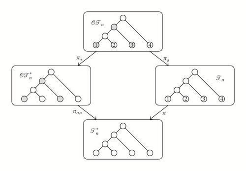
There exist natural isomorphism-preserving forgetful mappings
that “forget” the orderings or the labels of the trees. In particular, we shall call the image of a cladogram under π its shape. Figure 1 depicts an example of images under these forgetful mappings.
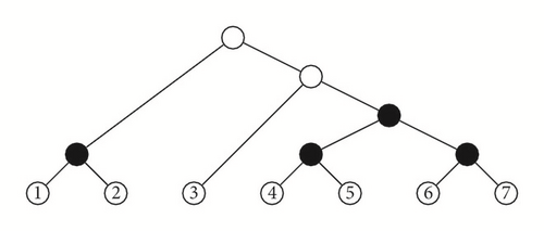
A symmetric branch point in a tree T is an internal node v such that if v1 and v2 are its children, then the subtrees and of T rooted at them have the same shape. For instance, the symmetric branch points in the cladogram depicted in Figure 2 are those filled in black.
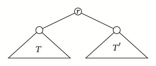
Given two cladograms T and T′ on Σ and Σ′, respectively, with Σ∩Σ′ = ∅, their root join is the cladogram T⋆T′ on Σ ∪ Σ′ obtained by connecting the roots of T and T′ to a (new) common root r; see Figure 3. If T, T′ are ordered cladograms, T⋆T′ is ordered by inheriting the orderings on T and T′ and ordering the children of the new root r as . If T and T′ are tree shapes, a similar construction yields a tree shape T⋆T′; if they are moreover ordered, then T⋆T′ becomes an ordered tree shape as explained above.
2.2. The α-Model
Ford’s α-model [4] defines, for every n⩾1, a family of probability density functions on that depends on one parameter α ∈ [0,1], and then it translates this family into three other families of probability density functions Pα,n on , on , and on , by imposing that the probability of a tree shape is equally distributed among its preimages under π, πo,∗, and π∘πo = πo,∗∘π∗, respectively.
- (1)
if T1 and T2 denote, respectively, the only cladograms in and , let ;
- (2)
for every m = 3, …, n, let be obtained by adding a new leaf labeled m to Tm−1. Then
(2) - (3)
When the desired number n of leaves is reached, the probability of every tree shape is defined as
(3)
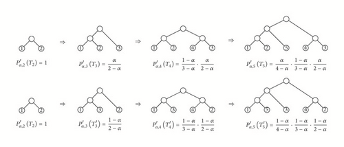
For instance, Figure 4 shows the construction of two cladograms in with the same shape and how their probability is built using the recursion in Step (2). If we generate all cladograms in with this shape, we compute their probabilities , and then we add up all these probabilities, we obtain the probability of this shape, which turns out to be 2(1 − α)/(4 − α); cf. [4, Figure 23].
- (i)
For every , if and it has k symmetric branch points, then
(4) -
because |π−1(T∗)| = n! /2k (see, e.g., [4, Lemma 31]).
- (ii)
For every , if , then
(5) -
because (T has 2n−1 different preimages under πo, obtained by taking all possible different combinations of orderings on the n − 1 sets child(v), v ∈ Vint(T∗)).
- (iii)
For every , if and it has k symmetric branch points, then
(6) -
because (from the 2n−1 possible preimages of T∗ under πo,∗, defined by all possible different combinations of orderings on the n − 1 sets child(v), v ∈ Vint(T∗), those differing only on the orderings on the children of the k symmetric branch points are actually the same ordered tree shape).
Proposition 1. For every 0 < m < n and for every and ,
3. Main Results
Our first result is an explicit formula for Pα,n(T), for every n⩾1 and .
Proposition 2. For every , its probability under the α-model is
Proof. Given , let To be any ordered cladogram such that πo(To) = T, and let and . If T∗ has k symmetric branch points, then, by (4), (6), and (10),
Remark 3. Ford states (see [4, Proposition 32 and page 30]) that if , then
As a second reason, which can be checked using a symbolic computation program, let us mention that if we take expression (22) as the probability of and hence of all other cladograms with its shape, and we assign to all other cladograms in the probabilities computed with Proposition 2, which agree on them with the values given by (19) (they are also provided in the aforementioned document ProblsAlpha.pdf), these probabilities do not add up 1.
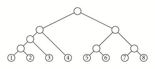
Combining Proposition 2 and (4) we obtain the following result.
Corollary 4. For every with k symmetric branch points,
This formula does not agree, either, with the one given in [4, Proposition 29]: the difference lies again in the same factor of 2 to the power of the number of internal nodes that are not symmetric branch points but whose children have the same number of descendant leaves.
The family of density mappings (Pα,n) n satisfies the following Markov branching recurrence.
Corollary 5. For every 0 < m < n and for every and ,
Proof. If and , then
Remark 6. Against what is stated in [4], does not satisfy any Markov branching recurrence; that is, there does not exist any symmetric mapping such that, for every k, l⩾1 and for every and ,

Data Availability
The data used to support the findings of this study are available at the Github page that accompanies this paper.
Conflicts of Interest
The authors declare that there are no conflicts of interest regarding the publication of this paper.
Acknowledgments
This research was supported by Spanish Ministry of Economy and Competitiveness and European Regional Development Fund Project DPI2015-67082-P (MINECO/FEDER). The authors thank G. Cardona and G. Riera for several comments on the SageMath module that accompanies this paper.


