Global Stability of Nonlinear Stochastic SEI Epidemic Model with Fluctuations in Transmission Rate of Disease
Abstract
We derive and analyze the dynamic of a stochastic SEI epidemic model for disease spread. Fluctuations in the transmission rate of the disease bring about stochasticity in model. We discuss the asymptotic stability of the infection-free equilibrium by first deriving the closed form deterministic (R0) and stochastic () basic reproductive number. Contrary to some author’s remark that different diffusion rates have no effect on the stability of the disease-free equilibrium, we showed that even if no epidemic invasion occurs with respect to the deterministic version of the SEI model (i.e., R0 < 1), epidemic can still grow initially (if ) because of the presence of noise in the stochastic version of the model. That is, diffusion rates can have effect on the stability by causing a transient epidemic advance. A threshold criterion for epidemic invasion was derived in the presence of external noise.
1. Introduction
Many mathematical models have been developed in order to understand disease transmissions and behavior of epidemics. Among these model is the SEI susceptible-exposed-infectious model. This model is used by some author in studying disease transmission of the Severe Acute Respiratory Syndrome (SARS) disease. Several authors [1–3] have studied other models like SEIR and SEIRS to analyze the spread of the disease. Guihua and Zhen [3] studied the deterministic SEI model by providing conditions for the global asymptotic stability of the infection-free and epidemic equilibrium using the higher dimensional Poincare-Bendixson property.
In this paper, we are interested in studying the effect of stochastic fluctuations in the disease transmission rates in the susceptible-exposed-infected epidemic model. We assume that a susceptible individual first goes through latent period after infection before becoming infectious. We consider a case where the disease is infectious in the latent period and the infected period. We study the role of external noise in the transmission rate. We assume the external noise is a Gaussian white noise. According to Méndez et al. [4], Langevin equations that describe system with real noise should be interpreted as a Stratonovich equation, instead of Ito equation. Due to this reason, we develop a Stratonovich stochastic dynamic SEI model by introducing noise in the transmission rates.
The paper is organized as follows.
In Section 2, we present a Stratonovich stochastic SEI model by allowing the transmission rates to fluctuate around a mean value. The Stratonovich model is now converted into its Ito version. In Section 3, we show that the solution of the stochastic SEI model discussed in Section 2 exists and it is positive. By linearizing the Ito version of the stochastic SEI model around the infection-free equilibrium, we give a closed form expectation of the susceptible, exposed and infected. In Section 4, the closed form value for the stochastic reproductive number is given. This is used to discuss and analyze the stability of the infection-free equilibrium. In Section 5, a numerical simulation is presented to verify our claim. The conclusion of the work is given in Section 6.
2. Stochastic SEI Model
We convert (8) to its Ito’s equivalent using the Stratonovich-Ito conversion (Bernardi et al. [6]) given below.
Theorem 1. The Ito Stochastic differential equation
3. Existence and Uniqueness of Positive Solution of (12)
In this section, we show that not only does the stochastic model (12) have a unique global solution but also the solution will remain within T whenever it starts from there.
Following Theorem 3.5 of Khasminskii [7], we use Theorem 4 below to show the existence and uniqueness of positive solution of (12).
Definition 2. Let C1,2(D) be the family of nonnegative functions V(t, u) defined on D such that they are continuously differentiable with respect to t and twice continuously differentiable with respect to u.
Definition 3. Define the domain Un by Un = {|x| < n}. One defines the differential operator L for a function V(t, u) ∈ C1,2 corresponding to a stochastic differential equation with drift and diffusion coefficients A(t, u) and B(t, u), respectively, by
Theorem 4. Suppose that (12) satisfies the classical existence and uniqueness theorem in every cylinder [a, b] × UR and, moreover, that there exists a nonnegative function such that for some constant c > 0
Proof. It is easy to show that (12) satisfies the classical existence and uniqueness theorem in every cylinder [a, b] × UR. Define by
It can be easily shown that Vn = inf|X|>nV(t, X) → ∞ as n → ∞. The result follows. The existence of E(t) = N − S(t) − I(t) follows immediately.
The fact that the solution (S, E, I) of (12) remains in T follows from Corollary 3.1 of Khasminskii [7].
3.1. Closed Form Expectation of Susceptible, Exposed, and Infected Population Near P0
We study the condition under which system (12) evolves into an endemic state by analyzing the endemic behavior of the linearized version of (12) around the infection-free equilibrium P0.
4. Stability Analysis of Infection-Free Equilibrium P0
Remark 5. It follows that (23) is equivalent to . We can rewrite in terms of R0 by combining (6) and (24) as follows:
Using the following theorem, we get conditions for stochastic asymptotic stability of the infection-free equilibrium.
Definition 6. The solution u(t) = 0 of system (20) is said to be
- (1)
p-stable (p > 0) for t ≥ 0, if
() - (2)
asymptotically p-stable, if it is p-stable and moreover as t → ∞;
- (3)
exponentially p-stable, if, for some positive constants A and c,
() - (4)
when p = 1, one says stability in the mean and for p = 2, one says stability in mean square.
Theorem 7. If
Proof. If (28) holds, it follows from (25) that R0 < 1 and (22) implies . If R0 > 1, then and as t → ∞.
Remark 8. Contrary to Remark 3.1 of Kim and Lin [1], if
Remark 9. Note that the global stability of the trivial solution u = 0 of (20) is equivalent to the global stability of the infection-free equilibrium P0 = (S∗, 0,0).
The following theorem shows that the expected value in (22) does not always converge to the trivial solution u = 0 of (20) if . In fact, if , then as t → ∞ if .
Proof. From (23) and (24), is equivalent to . If , then ν = (β2γ/(κ + μ + α2))S∗, z1 = μ, z2 = α2 + κ + μ + ν, z3 = 0, and as t → ∞, where c2 = −((γ + μ + α1)(κ + μ + α2)/γμ)m3S∗, . If m3 = 0, then as t → ∞.
We show the global stability of the infection-free equilibrium P0 and trivial solution u = 0 of the nonlinear stochastic systems (12) and (18), respectively.
Theorem 11. If the trivial solution u(t) = 0 for linear system (20) with drift and diffusion coefficients F(t, u) and G(t, u), respectively, is asymptotically stable and the drift and diffusion coefficients f(t, u) and g(t, u), respectively, of nonlinear system (18) satisfy the inequality
Proof. In a sufficiently small neighbourhood of u = 0, choose ϵ > 0 sufficiently small so that |u | < ϵ. We have
5. Numerical Simulations
Figure 1 verifies the global stability criteria discussed in Theorems 7, 10, and 11 and Remark 8.
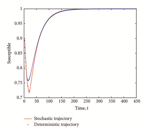
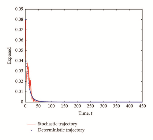
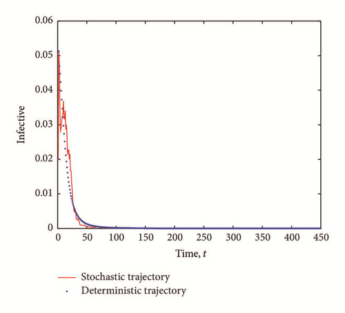
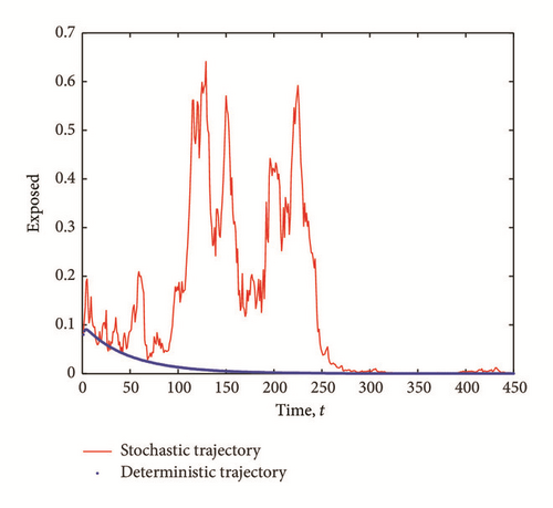
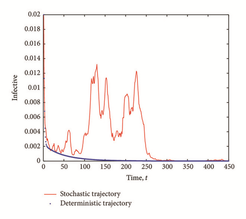
Figure 1 shows the graph of deterministic and stochastic trajectories of SEI model for initial conditions S0 = 0.9, E0 = 0.08, and I0 = 0.02. Here, we see that both R0 and are both less than one and both trajectories converge to the infection-free equilibrium (S∗, 0,0) = (1,0, 0).
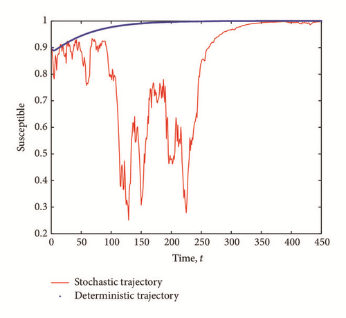
The transient epidemic advance is evident in all Figures 2(a), 2(b), and 2(c). The number of exposed (latent) individuals drastically increased for some time period. During the same period, the number of infected individuals increased and the number of susceptible individuals decreased.
6. Conclusion
The purpose of this work is to shed more light on the effects of the presence of external perturbations (in the form of white noise) in the disease transmission rates in a SEI model. By extending a SEI system of deterministic differential equations into a system of stochastic differential equations, we show the existence of solution of the stochastic model and derive the stochastic basic reproductive number, , corresponding to the deterministic reproductive number, R0. The stochastic basic reproductive number converges to the deterministic basic reproductive number R0 as the noise intensity σ1 tends to zero. We show that even if the infection-free equilibrium is stable, we might still have a transient epidemic advance. A condition in which this advance can happen is derived and analyzed. From our result, we conclude that the transient epidemic advance is induced by the noise intensity, σ1, of the white noise. It follows from (7) that as the noise intensity σ1 increases, the fluctuations around the mean number of infected individuals also increase thereby causing an initial epidemic growth provided that (29) is satisfied.
Competing Interests
The author declares that there is no conflict of interests regarding the publication of this paper.


