We consider a family of periodic SEIRS epidemic models with a fairly general incidence rate of the form Sf(I), and it is shown that the basic reproduction number determines the global dynamics of the models and it is a threshold parameter for persistence of disease. Numerical simulations are performed using a nonlinear incidence rate to estimate the basic reproduction number and illustrate our analytical findings.

1. Introduction

Epidemiological models in mathematics have been recognized as valuable tools in analyzing the dynamics of an infectious disease nowadays. They are used to describe the spread of disease and also to make control measures known to avoid its persistence, for example, via vaccination terms or treatment terms. These models consider the total population divided into compartments, given by the biological assumptions on the model and represented by functions depending on time t. The most common categories used are susceptible (S), infected (I), recovered (R), exposed (E), quarantined (Q), and vaccinated (V), and the dynamics of model is given by transmission rates from a compartment to another. We have then indicated that the models could be of type SIR, SIRS, SEIR, SEIRS, SEIVR, SEIQV, and so forth.

To ensure that the model can give a justified qualitative description of the disease, the choice of the incidence rate plays an important role. An incidence rate is defined as the number of new health related events or cases of a disease in a population exposed to the risk in a given time period. Some examples are the bilinear incidence rate, the saturated incidence rate, or a general incidence rate. The bilinear incidence rate has been repeatedly used by several authors. It is given by βSI, where β is the transmission rate and the product SI represents the contact between infected and susceptible individuals (based on the law of mass action). It was introduced by Kermack and McKendrick [1] in 1927, and even when it is mathematically simple to use, it faces multiple problems and challenges when it is used to describe disease propagation among gregarious animals or persons [2], because it goes to infinity when I becomes larger. In order to improve the modelling process to study the dynamics of infection among a large population, Capasso and Serio [3] in 1978 introduced a saturated incidence rate by studying the Cholera epidemic spread in Bari, given by βSI/(1 + kI), where β is the transmission rate and k the saturation constant. Unlike the bilinear incidence, saturated incidence does not grow up without a limit, but it goes to a saturation limit as I goes to infinity. Multiple types of saturated incidence have been used in the literature; see, for example, [2] for a list of them. To avoid the use of a single incidence function, the use of a general incidence rate that includes a family of particular functions with similar properties has become a topic of interest by several authors (see, e.g., [4–8]).

The basic reproduction (represented by ) is defined as “the average number of secondary cases produced by a single infected case when it is introduced in a susceptible population” and it has an important role in the study of disease transmission. In biological terms, usually when this number is less than one, the disease is eradicated from population, but when it is greater than one, the infection persists. Mathematically, it is of interest to compute a threshold parameter with the properties of the basic reproduction number. A method to compute this number for certain compartmental disease models is via the next-generation matrix method developed in [9]; however, it is not useful when the model presents time periodic seasonal terms. Authors like [10, 11] have defined its basic reproduction number for periodic models as an average, to give some results about extinction or persistence of infection. However Bacaër and Guernaouni in [12] introduced the definition of basic reproduction number for periodic environments, and, later, Wang and Zhao [13] made a formal definition of it, via the monodromy matrix.

In the present work, we focus on a family of SEIRS epidemic models with a time periodic seasonal term, improving the model of Moneim and Greenhalgh in [14], by introducing an incidence rate with a general function taken from [4] and the references therein.

We propose the following SEIRS model:

(1)

where N = S + E + I + R is the total population size, with S, E, I, R denoting the fractions of population that are susceptible, exposed, infected, and recovered, respectively. β(t) is the transmission rate and it is a continuous, positive T-periodic function. p (0 ≤ p ≤ 1) is the vaccination rate of all newborn children. r(t) is the vaccination rate of all susceptibles in the population and it is a continuous, positive periodic function with period LT, where L is an integer. μ is the common per capita birth and death rate. σ, γ, and δ are the per capita rates of leaving the latent stage, infected stage, and recovered stage, respectively. It is assumed that all parameters are positive constants.

Bai and Zhou in [5] answered some open problems stated in [14], they also showed that their condition is a threshold between persistence and extinction of the disease via the framework established in [13]. They assumed that the incidence was bilinear. In our study, the nonlinear assumptions on function f are listed below (see [4]).

(A1)
is continuously differentiable.
(A2)
f(0) = 0, f^′(0) > 0 and f(I) > 0 for all I > 0.
(A3)
f(I) − If^′(I) ≥ 0.

Under these assumptions, function f(I) includes various types of incidence rate; in particular, when f(I) = I, we are on the bilinear case considered in [14].

In addition, we assume the following extra conditions (see [15]).

(A4)
f^′′(0) ≤ 0.
(A5)
There exists ϵ^∗ > 0 such that when 0 < I < ϵ^∗, f(I) ≥ f(0) + If^′(0) + (1/2)I²f^′′(0).

This set of assumptions on the function f allows for more general incidence functions than the bilinear one, like saturated incidence functions and functions of the form βSI/(1 + kI^q); in particular, in the case when q > 1, they represent psychological or media effects depending on the infected population. In this last case the incidence function is nonmonotone on I. (A3) regulates the value of f(I) comparing it with the value at I of a line containing the origin of slope f^′(I) (note that this line varies as I increases), (A4) requires a concave f(I) at the origin, and (A5) imposes the geometrical condition that in a small neighborhood of the origin f(I) must lie between the tangent line of f at I and a concave parabola tangent to f at I.

We consider a family of SEIRS epidemic models with periodic coefficients and general incidence rate in epidemiology. Then we show that the global dynamics of solutions is determined by the basic reproduction number , generalizing the results in [5]. The layout of this paper is as follows: In Section 2, we prove the existence of a disease-free periodic solution and we introduce the basic reproduction number via the theory developed in [12, 13]. In Section 3, we adapt the arguments given in [5] to prove that the disease-free periodic solution of system (1) is globally asymptotically stable if and it is persistent when . Finally, in Section 4, we give some numerical simulations of our results, making a comparison between our basic reproduction number and the average reproduction number used by several authors (see, e.g., [10, 11]).

2. The Basic Reproduction Number

First of all, we prove nonnegativity of the solutions under nonnegative initial conditions.

Theorem 1. Let S₀, E₀, I₀, R₀ ≥ 0. The solution (S(t), E(t), I(t), R(t)) of (1) with

(2)

is nonnegative in the sense that S(t), E(t), I(t), R(t) ≥ 0, ∀t > 0, and satisfies S(t) + E(t) + I(t) + R(t) = N, with N constant.

Proof. Let N(t) = S(t) + E(t) + I(t) + R(t); then, adding all equations of system (1), we can see that dN/dt = 0, so the value of N is constant. Now, set x(t) = (S(t), E(t), I(t), R(t)) as the solution of system (1) under initial conditions x₀ = (S(0), E(0), I(0), R(0)) = (S₀, E₀, I₀, R₀) ≥ 0. By the continuity of solutions, for all of S(t), E(t), I(t) and R(t) that have a positive initial value at t = 0, we have the existence of an interval (0, t₀) such that S(t), E(t), I(t), R(t) ≥ 0 for 0 < t < t₀. We will prove that t₀ = ∞.

If S(t₁) = 0 for a t₁ ≥ 0 and other components of x(t) remain nonnegative at t = t₁, then

(3)

implying that whenever the solution x(t) touches the S-axis, the derivative of S is nondecreasing and the function S(t) does not cross to negative values. Similarly, when E(t₁) = 0 for a t₁ ≥ 0 and other components remain nonnegative, we have

(4)

When I(t₁) = 0 for a t₁ ≥ 0 and other components remain nonnegative,

(5)

Finally, when R(t₁) = 0 for a t₁ ≥ 0 and other components remain nonnegative,

(6)

Therefore, whenever x(t) touches any of the axes S = 0, E = 0, I = 0, or R = 0, it never crosses them.

In order to make the analysis of the model in a simpler way from now on, we make a reduction of dimension in system (1) making R = N − S − E − I, obtaining the following:

(7)

The dynamics of system (1) is equivalent to that of (7); moreover, due to positivity of solutions, we have S + E + I ≤ N, so we study the dynamics of system (7) in the region

(8)

A disease-free periodic solution can be found for (7). To find it, set E = I = 0; then, from the first equation of (7) we can obtain the following initial value problem:

(9)

From [5, 14], the equation above admits a unique positive LT-periodic solution given by

(10)

where

(11)

Therefore, is a disease-free periodic solution of (7); moreover, from [5] we have that ; therefore, lives in X.

Using the notation of [9], we sort the compartments so that the first two compartments correspond to infected individuals. Let x = (E, I, S) and define

(i)
: the rate of new infection in compartment i,
(ii)
: the rate of individuals into compartment i by other means,
(iii)
: the rate of individuals transfer out of compartment i.

System can be written as

(12)

where

(13)

Linearizing system (12) around the disease-free solution, we obtain the matrix of partial derivatives

, where

(14)

Using Lemma 1 of [9], we part

and

and set

(15)

For a compartmental epidemiological model based on an autonomous system, the basic reproduction number is determined by the spectral radius of the next-generation matrix FV⁻¹ (which is independent of time) [9]. The definition of basic reproduction number for nonautonomous systems has been studied for multiple authors; see, for example, [12, 13]. Particularly, Wang and Zhao in [13] extended the work of [9] to include epidemiological models in periodic environments. They introduced the next infection operator

given by

(16)

where C_LT is the ordered Banach space of all LT periodic functions from

, which is equipped with the maximum norm. ϕ(s) ∈ C_LT is the initial distribution of infectious individuals in this periodic environment, and Y(t, s), t ≥ s is the evolution operator of the linear periodic system:

(17)

meaning that, for each

, the 2 × 2 matrix Y satisfies

(18)

is the distribution of accumulative new infections at time t produced by all those infected individuals ϕ(s) introduced before t, with kernel K(t, a) = Y(t, t − a)F(t − a). The coefficient K_i,j(t, a) in row i and column j represents the expected number of individuals in compartment I_i that one individual in compartment I_j generates at the beginning of an epidemic per unit time at time t if it has been in compartment I_j for a units of time, with I₁ = E, I₂ = I [16].

Let r₀ > 0, r₀ is an eigenvalue of

if there is a nonnegative eigenfunction v(t) ∈ C_LT such that

(19)

Therefore, the basic reproduction number is defined as

(20)

the spectral radius of

. The basic reproduction number can be evaluated by several numerical methods and approximations [15–17]; in Section 4 we discuss this topic.

3. The Threshold Dynamics of R₀

3.1. Disease Extinction

Theorem 2. Let be defined as (20); then the disease-free periodic solution is asymptotically stable if and unstable if .

Proof. We use Theorem 2.2 of [13] and check conditions (A1)–(A7). Conditions (A1)–(A5) are clearly satisfied from the definitions of and given in Section 2. We prove only conditions (A6) and (A7). Define

(21)

and let Φ_M(t) be the monodromy matrix of system

(22)

(A6)
ρ(Φ_M(LT)) < 1. Let Ψ_M be a fundamental matrix for system dz/dt = M(t)z, with M defined as before and LT periodic; the monodromy matrix Φ_M(LT) is given by . The general solution of (22) is
(23)
so and . Note that , so Φ_M(LT) = Ψ_M(LT) and
(24)
Due to the fact that Φ_M(LT) is a constant, its eigenvalue is itself and ρ(Φ_M(LT)) < 1 for μ, δ, r(s) > 0.
(A7)
ρ(Φ_−V(LT)) < 1. Solving the system dz/dt = −V(t)z, we arrive at the general solution
(25)
so
(26)
Computing , we have
(27)
Clearly, ρ(Φ_−V(LT)) = max{e^−(μ+σ)LT, e^−(μ+γ)LT} < 1 for μ, γ, σ > 0.

Note 1. Due to the fact that Ψ_A is a fundamental solution of a periodic system, we can always choose it such that Ψ(0) = I, so the monodromy matrix satisfies Φ_A(LT) = Ψ_A(LT). This property is used in further analysis.

In order to prove the global stability of the disease-free periodic solution, we enunciate some useful definitions and some lemmas.

Let A(t) be continuous, cooperative, irreducible, and ω-periodic k × k matrix function, and Ψ_A(t) the fundamental matrix of system x^′(t) = A(t)x(t). Denote by ρ(Ψ_A(ω)) the spectral radius of Ψ_A(ω).

Lemma 3. Let p = (1/ω)ln⁡ρ(Ψ_A(ω)). Then there exists a positive, ω-periodic function v(t) such that e^ptv(t) is a solution of x^′(t) = A(t)x(t) (see proof in Lemma 2.1 of [18]).

Lemma 4. Function f(I) of model (1) satisfies f(I) ≤ f^′(0)I, ∀I ≥ 0.

Proof. Using assumptions on function f, we have

(28)

so function f(I)/I decreases ∀I > 0 and then

Lemma 5. Let (S(t), E(t), I(t)) be a solution of system (7) with initial conditions (S₀, E₀, I₀) ≥ 0, and the disease-free periodic solution of (7); then

(29)

Proof. Proof is similar to Lemma 4.1 of [14]. S(t) satisfies the first equation of system (7); then

(30)

Let

; then

(31)

Using Gronwall’s inequality

(32)

Taking limits in both sides, we obtain that

Now, we are able to enunciate our theorem for global stability of disease-free periodic solution.

Theorem 6. The disease-free periodic solution of system (7) is globally asymptotically stable if .

Proof. From Theorem 2 we have that is unstable for and asymptotically stable for , so it is sufficient to prove that any solution (S(t), E(t), I(t)) with nonnegative initial conditions (S₀, E₀, I₀) approaches as t tends to infinity.

Let ϵ > 0; from Lemma 5 we have

(33)

so there exists a N > 0 such that for all t₁ > N

(34)

which implies that

. Then, from the definition of supremum, we have that for all t > t₁

(35)

Then, we have proved that for all ϵ > 0 we can find a t₁ > 0 such that for all t > t₁.

Now, using Lemma 4, for ϵ > 0 we can find a t₁ > 0 such that for t > t₁

(36)

(37)

We consider the following perturbed subsystem:

(38)

which can be rewritten as

(39)

with F(t), V(t) defined in (15) and

(40)

Matrix (F − V + ϵH)(t) is LT-periodic, cooperative, irreducible, and continuous. Using Lemma 3, if q = (1/LT)ln⁡ρ(Ψ_F−V+ϵH(LT)), then there exists a positive and LT-periodic function v(t) = (v₁(t), v₂(t)) ^T such that e^qtv(t) is solution of system (38). Note that for all k > 0, function is also a solution of system (38) with initial condition kv(0) at t = t_i.

Choose a and α₁ > 0 such that ; then from (37) we have that

(41)

and using a comparison principle (see, e.g., [19] Theorem B.1), we have

for all

From Theorem 2.2 of [13], iff ρ(Φ_F−V(LT)) < 1. By the continuity of the spectrum for matrices (see [20], Section II.5.8), we can choose ϵ > 0 small enough so that ρ(Φ_F−V+ϵH(LT)) < 1 and then q < 0 (see Note 1). Thus, using positivity of solutions and comparison,

(42)

And similarly for I, we obtain that

(43)

We need only to prove that S(t) approaches . At disease-free periodic solution , where satisfies

(44)

Thus, R(t) = N − S(t) − E(t) − I(t) satisfies

(45)

Let ϵ₁ > 0 be arbitrary and r_max = max_u∈[0,LT]r(u). Due to (43) we can find a t₂ > 0 such that I(t) < ϵ₁ for t > t₂; moreover, we can find a t₃ > 0 such that for t > t₃. Then, let t₄ = max{t₂, t₃}; we have for t > t₄

(46)

Multiplying in both sides by e^(μ+δ)t and integrating from t₄ to t, we obtain

(47)

So, , where ϵ₁(r_max + γ)/(μ + δ) is arbitrarily small. Then , and using similar arguments for S and ϵ₂ > 0, we can find a t₅ > 0 with for t > t₅. Also, from (43), we can find t₆ > 0 with E(t) + I(t) < ϵ₂/2 for t > t₆, so, for t > max{t₅, t₆}, we have

(48)

Or, equivalently, , with ϵ₂ being arbitrarily small, and this implies that . We conclude by comparison and using Lemma 5 that , completing the proof.

Theorem 6 shows that disease will completely disappear as long as . Thus, reducing and keeping below the unity would be sufficient to eradicate infection, even in a periodic environment and a general incidence rate.

3.2. Disease Persistence

Uniform persistence is an important concept in population dynamics, since it characterizes the long-term survival of some or all interacting species in an ecosystem [21].

In this section we consider the dynamics of the periodic model when . We will show that actually is a threshold parameter for the extinction and the uniform persistence of the disease. Our results are inspired by [5, 15, 18, 22].

Let P : X → X be the Poincaré map associated with system (7); that is,

(49)

where X is defined in (8) and ϕ(t, x₀) is the unique solution of system (7) with ϕ(0, x₀) = x₀. We define the following sets:

(50)

Note that ∂X₀ is not the boundary of X₀, but it is a standard notation of persistence theory.

Lemma 7. Set X₀ is positively invariant under system (7).

Proof. Let x₀ = (S₀, E₀, I₀) ∈ X₀, that is, E₀ > 0, I₀ > 0, and let

(51)

be the solution of (7) with ϕ(0, x₀) = x₀. Due to nonnegativity of solutions and assumptions on function β(t) and f(I), we have

(52)

Using a comparison theorem (see, e.g., [19] Appendix B.1), we have for all t > 0

(53)

Similarly,

(54)

so,

(55)

Therefore, ϕ(t, x₀) remains on X₀ for all t > 0.

To use persistence theory developed in [21], we show that

(56)

where

(57)

Let x₀ = (S₀, 0,0) ∈ X and (S(t), E(t), I(t)) be the solution that passes through that initial condition. We have that ϕ(t, x₀) = (S₁(t), 0,0), with S₁(t) being a solution of (9) and S₁(0) = S₀ being a solution that satisfies the initial condition. By uniqueness of solutions we have E(t) = 0 = I(t) ∀ t ≥ 0, so x₀ lives on M_∂.

Now, if x₀ ∈ M_∂, we want x₀ = (S₀, 0,0). We prove an equivalent sentence: if x₀ ∈ ∂X₀∖{(S, 0,0) : S ≥ 0}, then it does not belong to M_∂. Consider an initial point x₀ = (S₀, E₀, I₀) ∈ ∂X₀∖{(S, 0,0) : S ≥ 0}; then E₀ > 0, I₀ = 0, or E₀ = 0, I₀ > 0. Suppose that E > 0 and I₀ = 0; then ϕ(t, x₀) holds

(58)

By continuity of E(t) and sign of derivative of I, we have that, for small 0 < t ≪ 1, E(t) > 0, I(t) > 0, so, for 0 < t ≪ 1, ϕ(t, x₀) ∈ X₀. Using invariance of X₀ (Lemma 7) we have ϕ(t, x₀) ∈ X₀ for all t > 1. Finally, for a m > 0 such that mLT > 1, we have P^m(x₀) = ϕ(mLT, x₀) ∈ X₀ and this implies (56). By the existence of a disease-free periodic solution (proved in Section 2), it is clear that there is one fixed point of P in M_∂ given by ([23]).

Now, we are in a position to introduce the following result of uniform persistence of the disease.

Theorem 8. Let ; then there exists an ϵ > 0 such that any solution (S(t), E(t)I(t)) of (7) with initial values (S(0), E(0), I(0)) ∈ X₀ satisfies

(59)

Proof. We first prove that P is uniformly persistent (see Definition 1.3.2 from [21]) with respect to (X₀, ∂X₀), because this implies that the solution of (7) is uniformly persistent with respect to (X₀, ∂X₀) (see [21], Theorem 3.1.1). Clearly, X₀ is relatively open in X, so ∂X₀ is relatively closed.

Define

(60)

we show that W^s(M₀)∩X₀ = ∅.

By Theorem 2.2 of [13], if and only if r(Ψ_F−V(LT)) > 1. Choose an η > 0 small enough with the property (see Appendix A). For α > 0, let us consider the following perturbed equation:

(61)

System above admits a unique positive LT-periodic solution of the form

(62)

whit

, which is globally attractive for all solutions of (61) (see Appendix B for proof), and with

(63)

Since is continuous in α, for all ϵ > 0 there is a δ > 0 such that for |α | < δ we have . Moreover, by continuity of solutions with respect to initial values we can find for all an such that if , then

(64)

Therefore, for η established before, we can find α small enough such that , ∀t > 0.

Again, by continuity of solutions with respect to initial values, for this small α > 0, there exists a δ > 0 such that for all (S₀, E₀, I₀) ∈ X₀ with ‖(S₀, E₀, I₀) − M₀‖ ≤ δ we have ‖ϕ(t, (S₀, E₀, I₀)) − ϕ(t, M₀)‖ < α, ∀t ∈ [0, LT].

We now claim that

(65)

By contradiction, suppose that

(66)

Without loss of generality, we can assume that ‖P^m(S₀, E₀, I₀) − M₀‖ < δ for all m ≥ 0 (see Appendix C). From the discussion above, ‖ϕ(t, P^m(S₀, E₀, I₀)) − ϕ(t, M₀)‖ < α, ∀m ≥ 0 and t ∈ [0, LT].

For any t ≥ 0, let t = mLT + t₁, where t₁ ∈ [0, LT) and m = [t/LT] is the greatest integer less than or equal to t/LT. Then, we get

(67)

If we set ϕ(t, (S₀, E₀, I₀)) = (S(t), E(t), I(t)), then we have E(t) ≤ α, I(t) ≤ α, ∀t ≥ 0, and from the first equation of (7) and Lemma 4 we arrive at

(68)

which is exactly the equation in (61). Since the unique periodic solution of (61) is globally attractive, we have for

solution of (61) that

. So for η given before, there exists T > 0 such that for all t ≥ T

(69)

or equivalently

. Moreover, from previous analysis,

; therefore, using comparison principle on (68) we arrive at

(70)

for t > T.

We have E(t), I(t) ≤ α, and α is fixed small, so we can take α < ϵ^∗ and use assumption (A5) in Introduction (see Appendix D) to obtain

(71)

where F, V are defined in (15), H is defined in (40), and

(72)

By Theorem 2.2 of [13], we have iff ρ(Φ_F−V(LT)) > 1. By continuity of spectrum (see [20] Section II), we can find α, ϵ such that

(73)

Consider the auxiliary system

(74)

then, using Lemma 3 there exists a solution of (71) with the form

, with p₂ = (1/LT)ln⁡(ρ(Φ_{F−V−ηH−αK}(LT))) > 0. Choose a t₂ > T and a small number α₂ > 0 such that (E₂(t₂), I₂(t₂)) ^T ≥ α₂v₂(0). Using comparison principle we get

, which implies E(t) → ∞ and I(t) → ∞. This leads to a contradiction.

The claim above shows that P is weakly uniformly persistent with respect to (X₀, ∂X₀). Note that P has a global attractor (see Lemma 5). It follows that M₀ is an isolated invariant set in X, W^s(M₀)∩X₀ = ∅. Every orbit in M_∂ converges to M₀ and M₀ is acyclic. By the acyclicity theorem on uniform persistence for maps ([21] Theorem 1.3.1 and Remark 1.3.1), it follows that P is uniformly persistent with respect to (X₀, ∂X₀); that is, there exists ϵ > 0 such that any solution of (7) satisfies lim_t→∞E(t) ≥ ϵ, lim_t→∞I(t) ≥ ϵ.

4. Numerical Simulations

In this section we provide some numerical simulations to illustrate the results obtained in our theorems and compare them with previous results.

To improve previous models used in references, we use a particular function

(75)

which includes the case f(I) = I used in [5]. One can check that function (75) satisfies conditions (A1)–(A5). Using this function, system (7) is rewritten as

(76)

Set an initial population N = 2,200,000 and take time t in years. Suppose μ = 0.02 per year, corresponding to an average human life time of 50 years. Following [5] take the parameters as follows: σ = 38.5 per year, γ = 100 per year, p = 0.85, δ = 0, and a = 1. Choose the periodic transmission as β(t) = β₀ + 0.0002cos⁡(2πt), with β₀ being the transmission parameter, and the periodic vaccination rate r(t) = 0.1 + 0.004cos⁡(2πt). Both functions have period LT = 1.

There exists multiple methods for computing the basic reproduction number, via numerical approximations, or finding a positive solution of the equation ρ(W(LT, 0, λ)) = 1 (see Theorem 2.1 of [13]). In order to compare our work with previous works, we approximate the basic reproduction number with its average value

, used by several authors as the reproduction number (for example [10, 11]), so define

(77)

where V is given by (15) and

(78)

with

being the average of functions

defined as

. Computing each average, we obtain

(79)

for β₀ ∈ (0.001819272510, ∞).

Following Theorem 2.1 of [13], to compute

, let W(t, s, λ), t ≥ s, be the evolution operator of the system

(80)

that is, for each λ ∈ (0, ∞), dW(t, s, λ)/dt = (−V(t) + F(t)/λ)W(t, s, λ), ∀t ≥ s, and W(s, s, λ) = I_2×2. With this operator,

is the unique solution of ρ(W(LT, 0, λ)) = 1.

Example 1. To illustrate our results, fix β₀ = 0.0018. Computing , we have , which is a first approximation of R₀. To solve system (80) numerically, we substitute the terms of expression of in (10):

(81)

The previous integral cannot be computed analytically, so we approach using Taylor expansion around 0 (remember that we want so solve ρ(W(LT, 0, λ)) = 1, where LT = 1), so even when we cannot find an explicit expression for , the Taylor expansion is a good way to estimate it in (0,1). It could be of interest to also use an approach of around t = 1 and compare the results with those obtained in the present work (see Section 5 for a discussion about this topic).

Setting an initial value λ₀ = 0.98 and letting λ_i = λ₀ + i(0.0001), we solve system (80) numerically for each λ_i (using initial conditions w(0) = (1,0) and w(0) = (0,1), to satisfy W(0,0) = I_2×2), and compute ρ₁ = ρ(W(LT, 0, λ_i)) until ρ₁ ~ 1. With previous process we arrive at ρ₁ = 1.00120166209265 for λ = 0.9872 and ρ₁ = 0.997826338969630 for λ = 0.9873; therefore . Using a finer step size 0.0000001 to have more accuracy, we arrive at .

Set initial values as S(0) = 1,500,000, E(0) = 400,000, I(0) = 40,000, and R(0) = N − (S(0) + E(0) + I(0)).

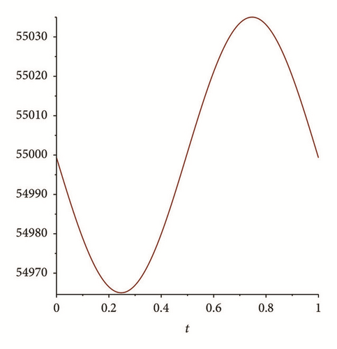
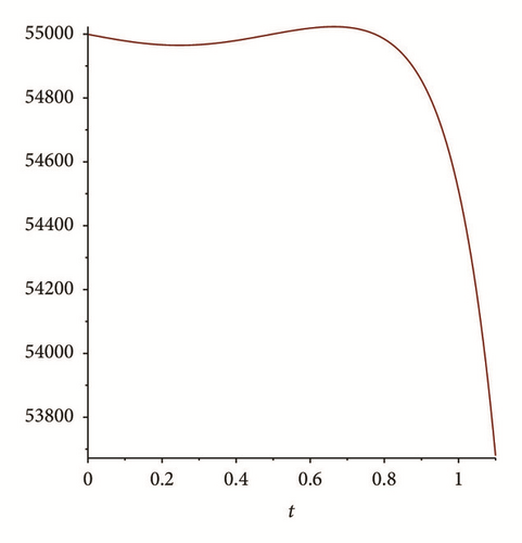
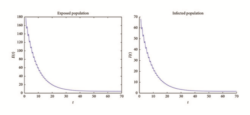
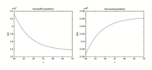
There exist multiple numerical methods to compute and plot the solutions of nonautonomous differential equations; see, for example, the Adomian method, the homotopy analysis method, or the modified homotopy methods (see, e.g., [24, 25]). For this work we use Matlab algorithms (ODE 45) to graph the solution of system (76) with these initial conditions. Figures 2 and 3 shows the results. We can see that I(t), E(t) goes to zero, while S(t), R(t) tend to stabilize; also S(t) is tending to with values between 54,000 and 56,000 (see Figure 1); this shows the results obtained in Theorem 6.

Details are in the caption following the image — **Figure 1 (a)**
Open in figure viewer PowerPoint

S component of infection-free periodic solution. Time t is given in years. (a) , because it is a periodic function of period 1, is plotted only in [0,1]. (b) Taylor expansion of around t = 0 of order t¹⁰.

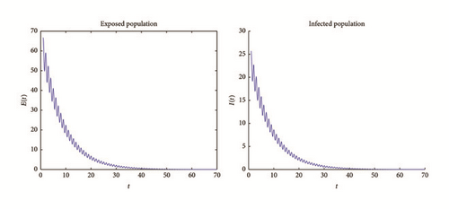
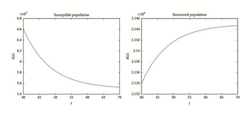
Example 2. Now, choose β₀ = 0.005. As we can see in Figures 4 and 5, the solutions of system (1) remain persistent when t tends to infinity; this fact suggests that from Theorem 8. In fact, if we compute the basic reproduction number and its average (using the process described in example 1), and ; therefore it is bigger than one. In fact, this shows the results of persistence obtained in Theorem 8.

5. Conclusion

In this paper we presented a model with seasonal fluctuation with a general incidence function Sf(I) that includes the bilinear case βSI (studied by [5]) and a family of saturated incidence rate of the form βSI/(1 + kI^q). We proved the existence of a disease-free periodic solution and defined the basic reproduction number , proving that it is a threshold parameter for disease, in the sense that when , the disease-free periodic solution is globally asymptotically stable, and when , the disease is persistent. A next step of this work is to consider a family of incidence rates more generally, changing Sf(I) by f(S, I) and trying to obtain results of persistence and stability similar to the ones obtained in this work. Another interesting topic is to ask what the behavior of system at is, in order to complete the analysis that we have made.

Several authors (e.g., [10, 11]) define as an average, which we denoted as to distinguish between it and the basic reproduction number defined by [13], via the monodromy matrix (which is a real threshold parameter for extinction and persistence of disease). We compute , approximate (with the help of Taylor theorem), and compare these values, obtaining that is not equal to ; moreover in both examples (similar comparisons can be observed also in the works made by [13, 17]). This fact suggests that the use of for persistence overestimates the threshold. To emphasize this conclusion, it would be helpful to find an example where but and then compute the solutions to observe the behavior (we affirm that the disease will go extinct due to Theorem 6).

To obtain the estimation of we used a code in Maple, which is based on numerical computing of ρ₁ = ρ(W(LT, 0, λ_i)) until ρ₁ ~ 1, where λ_i = λ₀ + Δ_λi, Δ_λ is the step size, and the initial estimation λ₀ is taken as . For this approximation we have used a Taylor expansion of the periodic solution ; another interesting possibility could be varying the approximation used for , for example, changing the Taylor approach of around t = 1 instead of t = 0. The graphs of the solutions were obtained with ODE 45 from Matlab, but other methods can be used to improve them, for example, Adomian methods or homotopy methods [24, 25]. The Maple code used to estimate is available for anyone who wants to use it.

Conflicts of Interest

The authors declare that they have no conflicts of interest.

Acknowledgments

This article was supported in part by Mexican SNI under Grants nos. 15284 and 33365.

Appendix

A. Assumption on η Used in Theorem 8

Note that has a positive minimum value (it is periodic, positive, and continuous, so it is bounded for t ∈ [0, LT] and then for all t > 0) and we can choose a η > 0 with the property , sufficiently small such that .

B. Periodic Solution of (61)

For each α, (61) used in the proof of Theorem 8 is

(B.1)

Solving the equation above, we arrive at the general solution

(B.2)

where p(s) = β(s)f^′(0)α + μ + r(s) + δ. We shall examine the behavior of an arbitrary solution

. For each n = 0,1, …, we can use an initial time

with initial point

and see that

(B.3)

Since p(s) is a periodic function,

(B.4)

where s − nLT ≥ t₀. Then

(B.5)

And using the change of variable u = s − LT, we have

(B.6)

Equation (B.6) gives a recursive relationship between the solution at t₀ + nLT and after LT times. If we set

, then for each solution

this relationship is described by

(B.7)

with F being on the right side of (B.6). If we take S_i and S_j, two different values of S_n, then

(B.8)

Then, F(S) is a contracting map, and by Banach fixed point theorem F has a unique fixed point S_i such that S_i+1 = F(S_i) = S_i or, equivalently,

. This fixed point can be found for any S that is a solution of a differential equation with arbitrary initial condition S(t₀) at any time t₀. The fixed point has the form

(B.9)

Thus, define the function

(B.10)

is a periodic function with period LT and is continuously differentiable with respect to t. One can check (by computing the derivative) that

is a solution of differential equation, so by existence and uniqueness of solutions it can be rewritten as

(B.11)

with initial condition

(B.12)

If we suppose the existence of another periodic solution

, then using (B.6) we arrive at

, by uniqueness of solutions

, and the periodic solution is unique. Computing the difference

, we have

(B.13)

so,

. Therefore, every solution

converges to

C. Assumption on P^m Used in Theorem 8

Let f(m)≔‖P^m(S₀, E₀, I₀) − M_i‖. If

(C.1)

then we have L = lim_m→∞(sup_n≥mf(n)) < δ. For all ϵ > 0 there exists a M_ϵ > 0 such that if m ≥ M_ϵ, then −ϵ < sup_n≥mf(n) − L < ϵ. In particular, for ϵ = (δ − L)/2 > 0 we have

(C.2)

or, equivalently, sup_n≥mf(n) < δ for m ≥ M_δ−L. Moreover, for all n ≥ m with m ≥ M_δ−L, we have f(n) < sup_n≥mf(n) < δ. Therefore, ‖Pⁿ(S₀, E₀, I₀) − M_i‖ < δ,

We can take

as initial condition and, therefore,

(C.3)

making our assumption valid.

So, we can assume without loss of generality that ‖P^m(S₀, E₀, I₀) − M_i‖ < δ for all m ≥ 0.

D. Expression (71)

From system (7) dE/dt = β(t)Sf(I)−(μ + σ)E, with

for t > T, so

(D.1)

Using assumption (A5) for f(I) and positivity of

, we have also

(D.2)

Therefore,

(D.3)

0 < I < α and f^′′(0) ≤ 0, so I² < αI and f^′′(0)I² ≥ f^′′(0)αI; applying this we arrive at

(D.4)

This expression can be written as (71).

References

1 Kermack W. O. and McKendrick A. G., A contribution to the mathematical theory of epidemics, Proceedings of the Royal Society A Mathematical, Physical and Engineering Sciences. (1927) 115, no. 772, 700–721, https://doi.org/10.1098/rspa.1927.0118, JFM53.0517.01.
10.1098/rspa.1927.0118
Google Scholar
2 Wang L., Zhang X., and Liu Z., An SEIR Epidemic Model with Relapse and General Nonlinear Incidence Rate with Application to Media Impact, Qualitative Theory of Dynamical Systems. 1–21, https://doi.org/10.1007/s12346-017-0231-6.
10.1007/s12346-017-0231-6
Web of Science® Google Scholar
3 Capasso V. and Serio G., A generalization of the Kermack-McKENdrick deterministic epidemic model, Mathematical Biosciences. (1978) 42, no. 1-2, 43–61, MR529097, https://doi.org/10.1016/0025-5564(78)90006-8, Zbl0398.92026, 2-s2.0-0018041874.
10.1016/0025-5564(78)90006-8
Web of Science® Google Scholar
4 Bai Z., Threshold dynamics of a periodic SIR model with delay in an infected compartment, Mathematical Biosciences and Engineering. (2015) 12, no. 3, 555–564, https://doi.org/10.3934/mbe.2015.12.555, MR3311724.
10.3934/mbe.2015.12.555
PubMed Web of Science® Google Scholar
5 Bai Z. and Zhou Y., Global dynamics of an SEIRS epidemic model with periodic vaccination and seasonal contact rate, Nonlinear Analysis: Real World Applications. (2012) 13, no. 3, 1060–1068, https://doi.org/10.1016/j.nonrwa.2011.02.008, MR2863936.
10.1016/j.nonrwa.2011.02.008
Web of Science® Google Scholar
6 Kaddar A., Elkhaiar S., and Eladnani F., Global Asymptotic Stability of a Generalized SEIRS Epidemic Model, Differential Equations and Dynamical Systems. 1–11, https://doi.org/10.1007/s12591-016-0313-y.
10.1007/s12591-016-0313-y
Web of Science® Google Scholar
7 Khan M. A., Khan Y., Badshah Q., and Islam S., Global stability of SEIVR epidemic model with generalized incidence and preventive vaccination, International Journal of Biomathematics. (2015) 8, no. 6, 2-s2.0-84944461154, https://doi.org/10.1142/S1793524515500825, 1550082, Zbl1356.92083.
10.1142/S1793524515500825
Web of Science® Google Scholar
8 Khan M. A., Khan Y., Khan T. W., and Islam S., Dynamical system of a SEIQV epidemic model with nonlinear generalized incidence rate arising in biology, International Journal of Biomathematics. (2017) 10, no. 7, 1750096, MR3705057.
10.1142/S1793524517500966
Web of Science® Google Scholar
9 van den Driessche P. and Watmough J., Reproduction numbers and sub-threshold endemic equilibria for compartmental models of disease transmission, Mathematical Biosciences. (2002) 180, no. 1, 29–48, https://doi.org/10.1016/S0025-5564(02)00108-6, MR1950747.
10.1016/S0025-5564(02)00108-6
CAS PubMed Web of Science® Google Scholar
10 Li L., Bai Y., and Jin Z., Periodic solutions of an epidemic model with saturated treatment, Nonlinear Dynamics. (2014) 76, no. 2, 1099–1108, 2-s2.0-84899645912, https://doi.org/10.1007/s11071-013-1193-0, Zbl1306.92060.
10.1007/s11071-013-1193-0
Web of Science® Google Scholar
11 Xu Y. and Li L., Global exponential stability of an epidemic model with saturated and periodic incidence rate, Mathematical Methods in the Applied Sciences. (2016) 39, no. 13, 3650–3658, MR3529375, https://doi.org/10.1002/mma.3812, 2-s2.0-84951765078.
10.1002/mma.3812
Web of Science® Google Scholar
12 Bacaër N. and Guernaoui S., The epidemic threshold of vector-borne diseases with seasonality. The case of cutaneous leishmaniasis in Chichaoua, Morocco, Journal of Mathematical Biology. (2006) 53, no. 3, 421–436, https://doi.org/10.1007/s00285-006-0015-0, MR2251779.
10.1007/s00285-006-0015-0
PubMed Web of Science® Google Scholar
13 Wang W. and Zhao X.-Q., Threshold dynamics for compartmental epidemic models in periodic environments, Journal of Dynamics and Differential Equations. (2008) 20, no. 3, 699–717, MR2429442, https://doi.org/10.1007/s10884-008-9111-8, Zbl1157.34041, 2-s2.0-47149095789.
10.1007/s10884-008-9111-8
Web of Science® Google Scholar
14 Moneim I. A. and Greenhalgh D., Use of a periodic vaccination strategy to control the spread of epidemics with seasonally varying contact rate, Mathematical Biosciences and Engineering. (2005) 2, no. 3, 591–611, MR2167668, https://doi.org/10.3934/mbe.2005.2.591, Zbl1079.92058.
10.3934/mbe.2005.2.591
PubMed Web of Science® Google Scholar
15 Posny D. and Wang J., Modelling cholera in periodic environments, Journal of Biological Dynamics. (2014) 8, no. 1, 1–19, MR3271014, https://doi.org/10.1080/17513758.2014.896482, 2-s2.0-84908024891.
10.1080/17513758.2014.896482
PubMed Web of Science® Google Scholar
16 Bacaër N., Approximation of the basic reproduction number R0 for vector-borne diseases with a periodic vector population, Bulletin of Mathematical Biology. (2007) 69, no. 3, 1067–1091, https://doi.org/10.1007/s11538-006-9166-9, MR2295844.
10.1007/s11538-006-9166-9
PubMed Web of Science® Google Scholar
17 Mitchell C. D., Reproductive Numbers for Periodic Epidemic Systems [PhD thesis], 2016, University of Texas, MR3611282.
Google Scholar
18 Zhang F. and Zhao X.-Q., A periodic epidemic model in a patchy environment, Journal of Mathematical Analysis and Applications. (2007) 325, no. 1, 496–516, MR2273541, https://doi.org/10.1016/j.jmaa.2006.01.085, 2-s2.0-33750325602.
10.1016/j.jmaa.2006.01.085
Web of Science® Google Scholar
19 Smith H. L. and Waltman P., The Theory of the Chemostat, 1995, Cambridge University Press, https://doi.org/10.1017/CBO9780511530043, MR1315301, Zbl0860.92031.
10.1017/CBO9780511530043
Google Scholar
20 Kato T., Perturbation Theory for Linear Operators, 1966, 132, Springer, New York, NY, USA, Grundlehren der Mathematischen Wissenschaften, MR0203473.
10.1007/978-3-642-53393-8
Google Scholar
21 Zhao X. Q., Dynamical Systems in Population Biology, 2003, Springer Science & Business Media, New York, NY, USA, https://doi.org/10.1007/978-0-387-21761-1, MR1980821.
10.1007/978-0-387-21761-1
Google Scholar
22 Yang Y., Ruan S., and Xiao D., Global stability of an age-structured virus dynamics model with Beddington-DeAngelis infection function, Mathematical Biosciences and Engineering. (2015) 12, no. 4, 859–877, MR3356515, https://doi.org/10.3934/mbe.2015.12.859, Zbl1330.35480, 2-s2.0-84927625725.
10.3934/mbe.2015.12.859
PubMed Web of Science® Google Scholar
23 Nakata Y. and Kuniya T., Global dynamics of a class of SEIRS epidemic models in a periodic environment, Journal of Mathematical Analysis and Applications. (2010) 363, no. 1, 230–237, https://doi.org/10.1016/j.jmaa.2009.08.027, MR2559058.
10.1016/j.jmaa.2009.08.027
Web of Science® Google Scholar
24 Khan Y. and Fardi M., A new efficient multi-parametric homotopy approach for two-dimensional Fredholm integral equations of the second kind, Hacettepe Journal of Mathematics and Statistics. (2015) 44, no. 1, 93–99, MR3363767, Zbl1322.65119, 2-s2.0-84961677927, https://doi.org/10.15672/HJMS.2015449096.
10.15672/HJMS.2015449096
Web of Science® Google Scholar
25 Khan Y., Sayevand K., Fardi M., and Ghasemi M., A novel computing multi-parametric homotopy approach for system of linear and nonlinear Fredholm integral equations, Applied Mathematics and Computation. (2014) 249, 229–236, MR3279416, https://doi.org/10.1016/j.amc.2014.10.070, Zbl1338.65285, 2-s2.0-84909642895.
10.1016/j.amc.2014.10.070
Web of Science® Google Scholar

Citing Literature

All articles

Global Dynamics of a Periodic SEIRS Model with General Incidence Rate

Abstract

1. Introduction

2. The Basic Reproduction Number

3. The Threshold Dynamics of R₀

3.1. Disease Extinction

3.2. Disease Persistence

4. Numerical Simulations

5. Conclusion

Conflicts of Interest

Acknowledgments

Appendix

A. Assumption on η Used in Theorem 8

B. Periodic Solution of (61)

C. Assumption on P^m Used in Theorem 8

D. Expression (71)

References

Citing Literature

Figures

References

Information

About Wiley Online Library

Help & Support

Opportunities

Connect with Wiley

Global Dynamics of a Periodic SEIRS Model with General Incidence Rate

Abstract

1. Introduction

2. The Basic Reproduction Number

3. The Threshold Dynamics of R0

3.1. Disease Extinction

3.2. Disease Persistence

4. Numerical Simulations

5. Conclusion

Conflicts of Interest

Acknowledgments

Appendix

A. Assumption on η Used in Theorem 8

B. Periodic Solution of (61)

C. Assumption on Pm Used in Theorem 8

D. Expression (71)

References

Citing Literature

Figures

References

Related

Information

3. The Threshold Dynamics of R₀

C. Assumption on P^m Used in Theorem 8