Volume 2017, Issue 1 2653124
Research Article
Open Access

Analysis of a Predator-Prey Model with Switching and Stage-Structure for Predator

T. Suebcharoen

Corresponding Author

T. Suebcharoen

Center of Excellence in Mathematics and Applied Mathematics, Department of Mathematics, Faculty of Science, Chiang Mai University, Chiang Mai 50200, Thailand cmu.ac.th

Search for more papers by this author
First published: 27 September 2017
Citations: 3
Academic Editor: Yuji Liu

Abstract

This paper studies the behavior of a predator-prey model with switching and stage-structure for predator. Bounded positive solution, equilibria, and stabilities are determined for the system of delay differential equation. By choosing the delay as a bifurcation parameter, it is shown that the positive equilibrium can be destabilized through a Hopf bifurcation. Some numerical simulations are also given to illustrate our results.

1. Introduction

The predator-prey system is important in dynamical population models and has been discussed by many authors [115].

In the related studies, a switching predator-prey model which has the switching property of predator was introduced by [7]. It was assumed that the predators catch prey in an abundant habitat. After a decrease in prey species population, the predator moves to another abundant habitat. In [8], the authors investigated a switching model of a two-prey one-predator system and they have shown that the system undergoes a Hopf bifurcation. They used the carrying capacity of prey as the bifurcations parameter. More examples on switching models can be found in [911]. Saito and Takeuchi [12] proposed a stage-structure model of a species’ growth consisting of immature and mature individuals. It is assumed that the predators are divided into two-stage groups: juveniles and adults. Only the adult predators are able to catch prey species. As for the juvenile predators, they live with the adult predators. It is assumed that juveniles survive on prey already caught by adults. They live on a different resource which is available in the abundant habitat from the adult predators. Consequently, stage-structure model is more realistic than the model without stage-structure. In [14], it was further assumed that the time from juveniles to adults is itself state dependent. Qu and Wei [15] studied the asymptotic behavior of a predator-prey model with stage-structure. They found that an orbitally asymptotically stable periodic orbit exists in that model.

The purpose of the present paper is to study nonlinear delayed differential equations each of which describes a switching and stage structured predator-prey model. The present paper is organized as follows. In the next section, the main mathematical model is formulated and the positivity and boundedness of solutions are presented. In Section 3, we discuss the local stability of equilibria by analyzing the corresponding characteristic equations and we prove the existence of Hopf bifurcations for the model. Finally, numerical results and a brief discussion are provided.

2. Model

In this paper, we extend the switching predator-prey model in [8] by introducing stage structured with time delay into the model. We consider the switching with stage-structure predator-prey model of the following form:
(1)
with initial conditions
(2)
The model is formulated under the following assumptions:
  • (1)

    It is assumed that two-prey species, denoted by x1 and x2, respectively, can be modelled by a logistic equation when the predator is absent. The parameter r is the prey intrinsic growth rate and k is its carrying capacity.

  • (2)

    The prey lives in two different habitats and each prey is able to migrate among two different habitats. The parameter p is the probability of successful transition from each habitat and q is inverse barrier strength in going out of the first habitat and the second habitat.

  • (3)

    The functions βx1/(x1 + x2) and βx2/(x1 + x2) have a characteristic property of a switching mechanism, where β is capturing rate.

  • (4)

    The parameter δ is the rate of conversion of prey to predator and μ is the death rate of predator.

  • (5)

    The predators are derived into two-stage groups: juveniles and adults, which are divided by age τ, and they are denoted by yj(t) and y(t), respectively. It is assumed that juveniles take τ units of time to mature and eγτ is the surviving rate of juveniles to adults. Notice, we assume that the juveniles suffer a mortality rate of γ.

For ecological reasons, we always assume that the initial data x1(θ), x2(θ), y(θ), yj(θ) ≥ 0 continuous on [−τ, 0), and x1(0), x2(0), y(0), yj(0) > 0. If (x1(t), x2(t), y(t), yj(t)) is a solution of system (1) through that initial data, it is easy to verify that (x1(t), x2(t), y(t), yj(t)) is positive on the maximum existence interval of solution. Such solutions will be called positive solution. Moreover, if such a solution is bounded above and below, it is called a positive solution. Furthermore, we discuss the bounded positive solutions of system (1) which implies a natural restriction; that is, our system (1) must have a bounded positive solution. The following theorem guarantees that our stage-structure predator-prey model (1) with initial condition (2) always has a bounded solution. Therefore, every solution to system (1) is positive and bounded.

Theorem 1. Every solution of system (1) with initial condition (2) is bounded for all t ≥ 0 and all of these solutions are ultimately bounded.

Proof. Let V(t) = γ(δx1 + δx2 + y + yj). By calculating the derivative of V(t) with respect to t along the positive solution of the system of system (1), we have

(3)
Let γ > μ. We have
(4)

Hence, there exists a positive constant C, such that

(5)
Thus, we get
(6)
Therefore, V(t) is ultimately bounded; that is, each solution of system (1) is ultimately bounded.

3. Local Stability and Existence of Hopf Bifurcation

The main goal in this section is to investigate the stability of a positive equilibrium and the existence of a Hopf bifurcation.

Because of the last equation of system (1), yj(t) is completely determined by x1(t), x2(t), y(t). Therefore, in the rest of this paper, we will study the following system:
(7)
with the initial conditions x1(θ), x2(θ), y(θ) ≥ 0 continuous on [−τ, 0) and x1(0), x2(0), y(0) > 0.
Before we proceed further, let us scale (7) by putting
(8)
and dropping the bars for the sake of simplicity. We obtain the following system containing dimensionless quantities:
(9)
Next, we find equilibria of system (9) by equating the derivatives on the left-hand sides to zero. The equilibria are solutions of the system
(10)
This gives two possible equilibria which are
  • (i)

    boundary equilibrium , which is corresponding to extinction of the predator, where is a real positive root of the cubic equation

    (11)

  • (ii)

    positive equilibrium , which is corresponding to coexistence of prey and predator and

    (12)

  • Here is a real positive root of the cubic equation

    (13)

  • or

    (14)

  • Obviously, is the one real positive root of   (13). The other two values of will be real and positive if

    (15)

We now analyze the stability of each equilibrium.
Let be any arbitrary equilibrium. The characteristic equation about E is given by
(16)

The next lemma gives conditions for the stability of equilibrium .

Theorem 2. The equilibrium is

  • (i)

    unstable if ;

  • (ii)

    locally asymptotically stable if

Proof. We consider the characteristic equation of (16) at the equilibrium E1. It follows that

(17)
Hence, one characteristic root is the solution of the equation
(18)

If , then , and f1(+) = . Therefore, f1(λ) has at least one positive root and the equilibrium E1 is unstable.

On the other hand, let ; that is,

(19)
Then f1(−) = − and f1(0) > 0. Thus, a root of f1(λ) has negative real part. Hence, the other characteristic roots are the solution of the equation
(20)
that is,
(21)
Since is a real positive root of the cubic equation , we have . We, then, consider the last few terms from (21)
(22)
Thus, all the roots of characteristic equation have negative real part. The equilibrium E1 is locally asymptotically stable.

Now, we analyze the stability of positive equilibrium . The associated characteristic equation is
(23)
where
(24)
In the following, we study the Hopf bifurcation for system (9), using the time delay τ as the bifurcation parameter. We assume that λ = iω  (ω > 0) is a root of the characteristic equation (23). Then we get
(25)
By separating real part and imaginary part, we obtain
(26)
By squaring both sides of the equations and using the property that sin2ωτ + cos2ωτ = 1, we can simplify the above equation. As a result,
(27)
Denote v = ω2, , , and . Then (27) becomes
(28)
By the Routh-Hurwitz criterion, we conclude that if
(29)
(23) has no positive real roots. Therefore, we get the following results.

Theorem 3. Suppose conditions in (29) hold and e1, e2 > 0, e3 ≥ 0. Then the equilibrium E2 is locally asymptotically stable.

Proof. For h(v) defined in (28), we have

(30)
and the zeros of (30) are
(31)
If e1, e2 > 0, then . Hence, v1 and v2 are negative. Thus, dh(v)/dv = 0 has no positive root. Since h(0) = e3 ≥ 0, it follows that h(v) = 0 has no positive roots. Therefore, the equilibrium E2 is locally asymptotically stable.

Theorem 4. Suppose that conditions in (29) hold and that

  • (i)

    either e3 < 0,

  • (ii)

    or e3 ≥ 0, e2 < 0, and ,

where ω0 satisfies G(iω0) = 0 with G given in (23). Then the equilibrium E2 is locally asymptotically stable if τ < τ0 and is unstable if τ > τ0, where
(32)
Furthermore, when τ = τ0, a Hopf bifurcation occurs; that is, a family of periodic solutions are bifurcated from E2 as τ passes through the critical value τ0.

Proof. If e3 < 0, then it follows from (28) that h(0) < 0 and limvh(v) = . Thus, (27) has at least one positive root. If e2 < 0, then is one positive root of dh(v)/dv = 0. Since h(0) = e3 ≥ 0, it follows that h(v) = 0 has at least one positive root. As a consequence, (27) has a positive root ω0. This implies that the characteristic equation (23) has a pair of purely imaginary roots.

Let u(τ) = η(τ) + iω(τ) be the eigenvalue of (23) such that η(τ0) = 0 and ω(τ0) = ω0. If there exists ω0 > 0, such that G(iω) = 0. Then by the first equation of (26), we have

(33)
and then
(34)
By taking the derivative of the characteristic equation (23) with respect to τ, we have
(35)
Thus,
(36)
We can also verify the following transversality condition [16]:
(37)
Therefore, if τ = τ0, then a Hopf bifurcation occurs; that is, a family of periodic solutions appear as τ passes through the critical value τ0.

4. Numerical Simulations and Discussion

In this section, we present some numerical simulation of system (9) at different parameters to illustrate our analytic results.

Example 5. Let g = 1.8  b = 0.6  α = 2  d = 3 and we consider the following system:
(38)
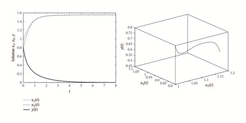
In this case, we obtain only one boundary equilibrium E1 = (1.556,1.557,0), and the conditions of (ii) in Theorem 2 are satisfied. Therefore, the equilibrium E1 is locally asymptotically stable. The behaviors of x1, x2, and y with respect to t are shown in Figure 1. According to the graph in Figure 1, the predator population decreases and eventually the predator species becomes extinct. As for prey species, the population of both species reaches the equilibrium as the predator population approaches zero.

Details are in the caption following the image
The behavior of x1, x2, and y with respect to t for Example 5.

Example 6. As an example, consider the following system:
(39)
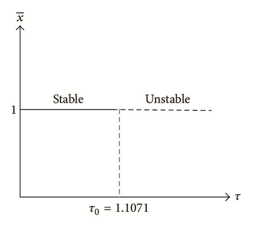
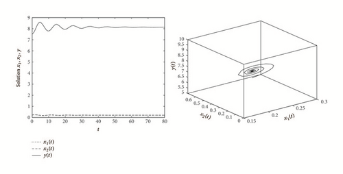
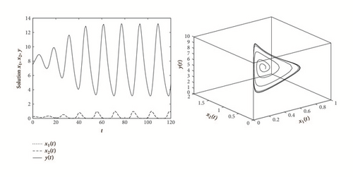
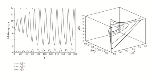
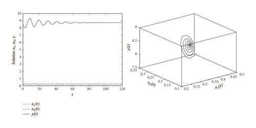
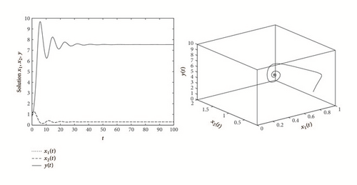
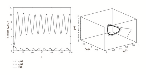
There is a positive equilibrium E2 = (0.3,0.3,7.53). By direct calculation, we have e3 = −0.01903, ω0 = 0.639, and . From Theorem 4, there is a critical value τ0 = 1.1071, and the equilibrium E2 is locally asymptotically stable as τ < τ0 = 1.1071. A Hopf bifurcation occurs as τ = τ0 = 1.1071 and the equilibrium becomes unstable and stable periodic solutions exist for τ > τ0 = 1.1071. Figures 2 and 3 show the solutions of that system corresponding to τ = 0.5 and τ = 1.8. Furthermore, a bifurcation diagram for Example 6 is shown in Figure 4. This is an example when the predator and prey coexist permanently. If the time that juvenile takes to be mature is less than τ0, then both predators and prey population reach the nonzero equilibrium. They can coexist permanently. On the other hand, if the time that juvenile predators takes to become mature and ready to hunt is longer than τ0, then the population of both predator and prey species becomes unstable and periodic.

Details are in the caption following the image
The behavior of x1, x2, and y with respect to t for Example 6 with τ = 0.5.
Details are in the caption following the image
The behavior of x1, x2, and y with respect to t for Example 6 with τ = 1.8.
Details are in the caption following the image
Bifurcation diagram for Example 6.

Example 7. As an example, consider the following system:
(40)
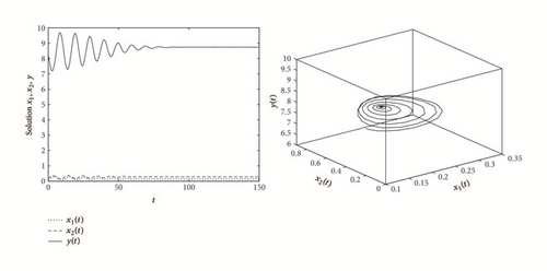
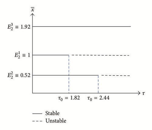
In this case, we obtain three positive equilibria , , and . By Theorem 4, we know that the positive equilibrium is locally asymptotically stable when τ < τ0 = 1.8227 and unstable when τ > τ0 = 1.8227, and the system can also undergo a Hopf bifurcation at the equilibrium when τ crosses through the critical value τ > τ0 = 1.8227; see Figures 5 and 6. Similarly, at the positive equilibrium , a Hopf bifurcation occurs as τ = τ0 = 2.4353. Hence, the positive equilibrium is locally asymptotically stable when τ < τ0 = 2.4353 and unstable when τ > τ0 = 2.4353; see Figures 7 and 8. For equilibrium , (27) has no positive real root. Hence, equilibrium is locally asymptotically stable and no stability switches can occur; see Figure 9. On this last example, what occurs at the first two equilibria and is similar to the previous example where Hopf bifurcations occur at τ0’s and the stable limit cycle exists. The predator and prey species coexist. As for the other equilibrium , the system is locally asymptotically stable where predator and prey species also coexist. Finally, the bifurcation diagram for Example 7 is shown in Figure 10.

Details are in the caption following the image
The behavior of x1, x2, and y with respect to t for equilibrium with τ = 0.6.
Details are in the caption following the image
The behavior of x1, x2, and y with respect to t for equilibrium with τ = 2.
Details are in the caption following the image
The behavior of x1, x2, and y with respect to t for equilibrium with τ = 1.8.
Details are in the caption following the image
The behavior of x1, x2, and y with respect to t for equilibrium with τ = 2.6.
Details are in the caption following the image
The behavior of x1, x2, and y with respect to t for equilibrium with τ = 2.6.
Details are in the caption following the image
Bifurcation diagram for Example 7.

5. Concluding Remarks

In this paper, we find that system (7) has complex dynamics behavior. By Theorem 2, our results show that the predator and prey coexist permanently if ; that is, the adult predators’ reproductive rate at the peak of prey abundance is larger than its death rate. On the other hand, the predator faces extinction, if , which implies that the predator’s possible highest reproductive rate is less than its death rate. We also find the stability switches of the positive equilibrium E2 due to the increase of τ. Our results show that when there is no time delay or the time delay is very small, the positive equilibrium E2 is locally asymptotically stable. As the time delay increases to the critical value, it can cause a stable equilibrium to become unstable and Hope bifurcation can occur.

Conflicts of Interest

The author declares that there are no conflicts of interest regarding the publication of this article.

Acknowledgments

This research was supported by Chiang Mai University, Thailand.

      The full text of this article hosted at iucr.org is unavailable due to technical difficulties.