International Journal of Differential Equations

Volume 2017, Issue 1 1467049

Research Article

Open Access

Identifying Initial Condition in Degenerate Parabolic Equation with Singular Potential

K. Atifi

orcid.org/0000-0001-6425-0015

Laboratoire de Mathématiques, Informatique et Sciences de l’Ingénieur (MISI), Université Hassan 1er, 26000 Settat, Morocco uh1.ac.ma

Search for more papers by this author

Y. Balouki,

Y. Balouki

Laboratoire de Mathématiques, Informatique et Sciences de l’Ingénieur (MISI), Université Hassan 1er, 26000 Settat, Morocco uh1.ac.ma

Search for more papers by this author

El-H. Essoufi,

El-H. Essoufi

Laboratoire de Mathématiques, Informatique et Sciences de l’Ingénieur (MISI), Université Hassan 1er, 26000 Settat, Morocco uh1.ac.ma

Search for more papers by this author

B. Khouiti,

Corresponding Author

B. Khouiti

[email protected]

orcid.org/0000-0003-1725-7147

Laboratoire de Mathématiques, Informatique et Sciences de l’Ingénieur (MISI), Université Hassan 1er, 26000 Settat, Morocco uh1.ac.ma

Search for more papers by this author

K. Atifi,

K. Atifi

orcid.org/0000-0001-6425-0015

Laboratoire de Mathématiques, Informatique et Sciences de l’Ingénieur (MISI), Université Hassan 1er, 26000 Settat, Morocco uh1.ac.ma

Search for more papers by this author

Y. Balouki,

Y. Balouki

Laboratoire de Mathématiques, Informatique et Sciences de l’Ingénieur (MISI), Université Hassan 1er, 26000 Settat, Morocco uh1.ac.ma

Search for more papers by this author

El-H. Essoufi,

El-H. Essoufi

Laboratoire de Mathématiques, Informatique et Sciences de l’Ingénieur (MISI), Université Hassan 1er, 26000 Settat, Morocco uh1.ac.ma

Search for more papers by this author

B. Khouiti,

Corresponding Author

B. Khouiti

[email protected]

orcid.org/0000-0003-1725-7147

Laboratoire de Mathématiques, Informatique et Sciences de l’Ingénieur (MISI), Université Hassan 1er, 26000 Settat, Morocco uh1.ac.ma

Search for more papers by this author

First published: 14 June 2017

https://doi.org/10.1155/2017/1467049

Citations: 2

Academic Editor: Jen-Chih Yao

Share a link

Email
Wechat
Bluesky

Abstract

A hybrid algorithm and regularization method are proposed, for the first time, to solve the one-dimensional degenerate inverse heat conduction problem to estimate the initial temperature distribution from point measurements. The evolution of the heat is given by a degenerate parabolic equation with singular potential. This problem can be formulated in a least-squares framework, an iterative procedure which minimizes the difference between the given measurements and the value at sensor locations of a reconstructed field. The mathematical model leads to a nonconvex minimization problem. To solve it, we prove the existence of at least one solution of problem and we propose two approaches: the first is based on a Tikhonov regularization, while the second approach is based on a hybrid genetic algorithm (married genetic with descent method type gradient). Some numerical experiments are given.

1. Introduction

The inverse problem is expressed when the PDE solution is measured or specified, and we are interested in determining some properties: coefficients, forcing term, boundary, or initial condition from the partial knowledge of the system in a limited time interval (see [1, 2]).

In the last recent years, an increasing interest has been devoted to degenerate parabolic equations. Indeed, many problems coming from physics (boundary layer models in [3], models of Kolmogorov type in [4], etc.), biology (Wright-Fisher models in [5] and Fleming-Viot models in [6]), and economics (Black-Merton-Scholes equations in [7]) are described by degenerate parabolic equations [8].

The identification of the initial state of nondegenerate parabolic problems is well studied in the literature (see [9–11]). However, as far as we know, the degenerate case has not been analysed in the literature.

In this paper, we are interested in estimating the initial condition by the variational method in data assimilation of degenerate/singular parabolic equation:

()

where Ω = ]0,1[, α ∈ ]0,1[, β ∈ ]0,2 − α[, λ ⩽ 0, and f ∈ L²(Ω × ]0, T[). With initial and boundary conditions

()

The mathematical model leads to a nonconvex minimization problem

()

where the functional J is defined as follows:

()

subject to ψ being the weak solution of the parabolic problem (1) with initial state u, ψ^obs an observation of ψ in Ω × ]0, T[, and C the observation operator. The space A_ad is the set of admissible initial states.

Problem (3) is ill-posed in the sense of Hadamard. To solve this problem, we propose two approaches.

The first approach is based on regularization, for the first time, applied to solve a degenerate inverse problem. The problem thus consists of minimizing a functional of the form

()

Here, the last term in (5) stands for the so-called Tikhonov-type regularization ([12, 13]), ε being a small regularizing coefficient that provides extra convexity to the functional J_T and ψ^b a priori (background) knowledge of the true state (the state to estimate). We consider that the values of ψ^b are given in each point of analysis grid-points.

The second approach is applied when there is a partial knowledge of values of ψ^b (example 20%); the regularization parameter is very difficult to determine. To overcome this problem, we propose a new approach, based on a hybrid genetic algorithm (married genetic with descent method gradient type). Finally, we make a comparison between the two mentioned approaches (with 20% of ψ^b).

First of all, we prove that problem (3) has at least one solution. The gradient of the functional J is calculated with the adjoint method. Numerical experiments are presented to show the performance of our approaches.

2. Problem Statement and Main Result

Consider the following problem:

()

where Ω = ]0,1[, f ∈ L²(Ω × ]0, T[),and A is the operator defined as

()

with α∈]0,1[, β∈]0,2 − α[, and λ ⩽ 0.

We want to estimate ψ₀ thanks to an observation ψ^obs(x, t) of ψ(x, t) in Ω × ]0, T[. The minimization problem associated with this problem is

()

where the functional J is as follows:

()

subject to ψ being the weak solution of the parabolic problem (6) with initial state u, ψ^b the background state, and C the observation operator. The space A_ad is the set of admissible initial states (will be defined later).

We now specify some notations we shall use. Let us introduce the following functional spaces (see [14–16]):

()

with

()

We recall that (see [16])

is an Hilbert space and it is the closure of

for the norm

. If

then the injections

()

are compacts.

Firstly, we prove that problem (6) is well-posed, the functional J is continuous, and J is G-derivable in A_ad.

The weak formulation of problem (6) is

()

Let

()

We discuss the following cases.

(1) Noncoercive Case (see [14], λ = 0). In this case, the bilinear form B becomes

()

We have a(x) = 0 at x = 0, from where the bilinear form B will be noncoercive.

Let

()

We recall the following theorem.

Theorem 1 (see [14], [17], [18].)For all f ∈ L²(Ω × ]0, T[) and ψ₀ ∈ L²(0,1), there exists a unique weak solution which solves problem (6) such that

()

and there is a constant C_T such that for any solution of (6)

()

if more

then

()

and there is a constant C_T such that

()

Theorem 2. Let ψ be the weak solution of (6) with initial state ψ₀. In noncoercive case, the function

()

is continuous, and the functional J has at least one minimum in A_ad.

Theorem 3. Let ψ be the weak solution of (6) with initial state ψ₀. The function

()

is G-derivable in A_ad.

(2) Subcritical Potential Case (see [19, 20], λ ≠ 0). Then the bilinear form B becomes

()

Since a(x) = 0 at x = 0 and lim_x→0⁡(λ/x^β) = +∞, the bilinear form B is noncoercive and is noncontinuous at x = 0.

Consider the not bounded operator (K, D(K)) where

()

Let

()

We recall the following theorem.

Theorem 4 (see [15], [19].)If f = 0 then, for all ψ₀ ∈ L²(Ω), problem (6) has a unique weak solution

()

if more ψ₀ ∈ D(K) then

()

if f ∈ L²(]0,1[×]0, T[) then, for all ψ₀ ∈ L²(Ω), problem (6) has a unique solution

()

Theorem 5. Let ψ be the weak solution of (6) with initial state ψ₀. In subcritical potential case, the function

()

is continuous, and the functional J is continuous in A_ad.

Theorem 6. Let ψ be the weak solution of (6) with initial state ψ₀. The function

()

is G-derivable in A_ad.

3. Proof

Proof of Theorem 2. Let be a small variation such that ψ₀ + δψ₀ ∈ A_ad.

Consider δψ = ψ^δ − ψ, with ψ being the weak solution of (6) with initial state ψ₀ and ψ^δ is the weak solution of (6) with initial state

Consequently, δψ is the solution of the variational problem:

()

Hence, δψ is the weak solution of (6) with f = 0. We apply the estimate in Theorem 1 with f = 0. This gives the following.

There is a constant C_T such that

()

therefore

()

And from (32) we have

()

Hence,

()

In addition, from (32) we have

()

Equations (34), (36), and (41) imply the continuity of the function

()

Hence, the functional J is continuous in

()

We have , where α∈]0,1[, which gives Since the set A_ad is bounded in , then A_ad is a compact in L²(Ω). Therefore, J has at least one minimum in A_ad.

Proof of Theorem 3. Let ψ₀ ∈ A_ad and δψ₀ such that ψ₀ + δψ₀ ∈ A_ad; we define the function

()

where δψ is the solution of the variational problem

()

and we pose

()

We want to show that

()

We easily verify that the function ϕ is solution of the following variational problem:

()

By the same way as that used in the proof of continuity, we deduce

()

Hence, the function φ : ψ₀ → ψ is G-derivable in A_ad and we deduce the existence of the gradient of the functional J.

Proof of Theorem 5. Let δψ₀ ∈ L²(Ω) be a small variation such that ψ₀ + δψ₀ ∈ A_ad.

Consider δψ = ψ^δ − ψ, with ψ being the weak solution of (6) with initial state ψ₀, and ψ^δ is the weak solution of (6) with initial state .

Consequently, δψ is the solution of variational problem

()

Take v = δψ; this gives

()

since Ω is independent of t, which gives

()

By integrating between 0 and t with t ∈ [0, T] we obtain

()

and since a(x)⩾0 and −λ/x^β > 0, ∀x ∈ Ω, we obtain

()

this gives

()

From where

()

Which gives the continuity of the function

()

Hence, the functional J is continuous in

()

Proof of Theorem 6. Let ψ₀ ∈ A_ad and δψ₀ such that ψ₀ + δψ₀ ∈ A_ad; we define the function

()

where δψ is the solution of the variational problem

()

and we pose

()

We want to show that

()

We easily verify that the function ϕ is the solution of the following variational problem:

()

By the same way as that used in the proof of continuity, we deduce

()

Hence, in all cases, the function φ : ψ₀ → ψ is G-derivable in A_ad and we deduce the existence of the gradient of the functional J.

Now, we are going to compute the gradient of J with the adjoint state method.

4. Gradient of J

We define the Gâteaux derivative of ψ at ψ₀ in the direction h ∈ L²(Ω), by

()

where ψ(ψ₀ + εh) is the weak solution of (6) with initial state ψ₀ + εh, and ψ(ψ₀) is the weak solution of (6) with initial state ψ₀.

We compute the Gâteaux (directional) derivative of (6) at ψ₀ in some direction h ∈ L²(Ω), and we get the so-called tangent linear model:

()

We introduce the adjoint variable P, and we integrate

()

Let us take P(x = 0) = P(x = 1) = 0; then we may write .

And with P(T) = 0 we may now rewrite (69) as

()

this gives

()

The Gâteaux derivative of the functional

()

at ψ₀ in the direction h ∈ L²(Ω) is given by

()

After some calculations, we arrive at

()

The adjoint model is

()

Problem (75) is retrograde; we make the change of variable t↔T − t, which gives

()

with

From (71), (74), and (75) the gradient of J is given by

()

With the change of variable t↔T − t, the gradient becomes

()

To calculate a gradient of J, we solve two problems: (6) and (76). The result solution of (6) is used in the second member of problem (76).

5. Discretization of Problem

Step 1 (full discretization). To resolve problem (6) and (76), we use the method θ-schema in time. This method is unconditionally stable for 1 > θ ≥ 1/2.

Let h be the steps in space and Δt the steps in time.

Let

()

we put

()

Let

()

Therefore,

()

is approximated by

()

Let us define

()

Letting , finally we get

()

where

()

Step 2 (discretization of the functional one has).

()

We recall that the method of Thomas Simpson to calculate an integral is

()

with x₀ = a, x_N+1 = b, x_i = a + ih, i ∈ {1, …, N + 1}.

Let the functions

()

This gives

()

where

()

with t₀ = 0, t_M+1 = T, t_j = jdt, j ∈ {1, …, M + 1}.

Therefore,

()

Step 3 (discretization of ∇J). The adjoint problem (76) is discretized as (85), so,

()

6. Numerical Experiments and Results

In this section, we discuss two cases:

In case we have a priori knowledge ψ^b of in each point of analysis grid-points, we apply the Tikhonov approach to solve the minimization problem (8). The data ψ^b is assumed to be corrupted by measurement errors, which we will refer to as noise. In particular, we suppose that . Here, we study the impact of err (err = ‖e‖₂) on the construction of the solution.

In case we have a partial knowledge of values of ψ^b (example 20%): firstly, we apply the hybrid approach to rebuild the initial state. Secondly, we make a comparison between both hybrid and Tikhonov approaches.

The tests have been performed in Matlab 2012A, on a Windows 7 platform.

6.1. Regularization Approach

The differentiability and continuity in A_ad of the functional,

()

is deduced from the differentiability and continuity of the functional J, and we have

()

where P is the solution of (76).

The main steps for descent method at each iteration are the following:

(i)
Calculate ψ^k solution of (6) with initial condition ψ₀.
(ii)
Calculate P^k solution of (76).
(iii)
Calculate the descent direction d_k = −∇J_T(ψ₀).
(iv)
Find t_k = argmin_t>0⁡J_T(ψ₀ + td_k)
(v)
Update the variable ψ₀ = ψ₀ + t_kd_k.

The algorithm ends when |J_T(ψ₀)| < μ, where μ is a given small precision.

t_k is chosen by the inaccurate linear search by Rule Armijo-Goldstein as follows:

let α_i, β ∈ [0,1[ and α > 0
if
t_k = α_i and stop
if not
α_i = αα_i.

We do all the tests on Pc with the following configurations: Intel Core i3 CPU 2.27 GHz; RAM = 4 GB (2.93 usable).

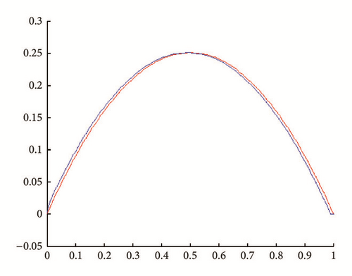
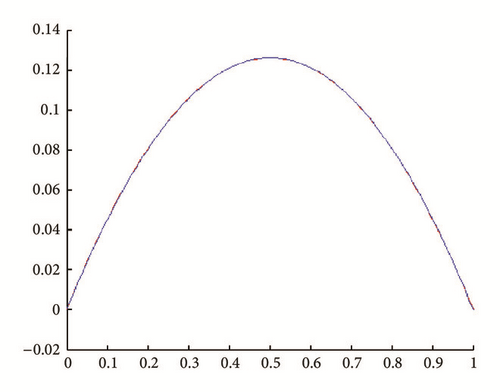
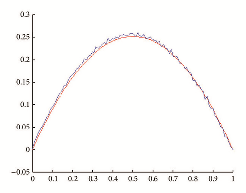
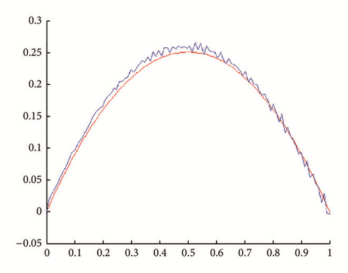
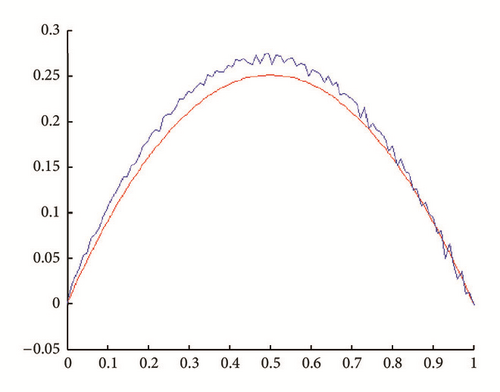
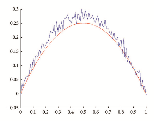
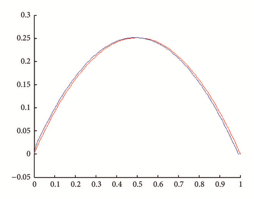
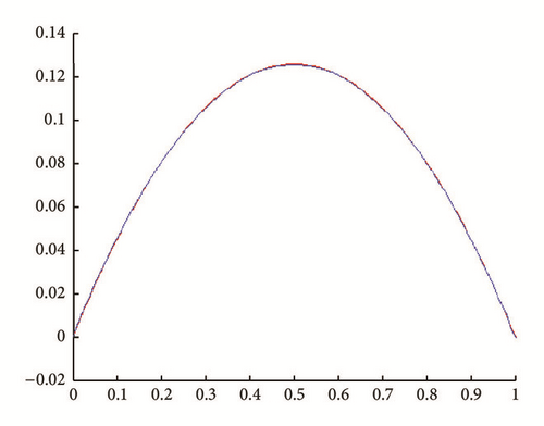
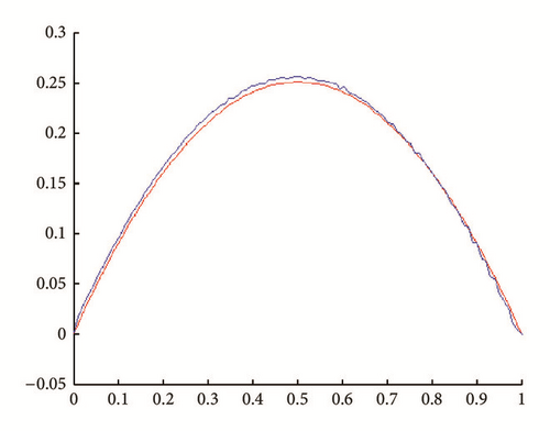
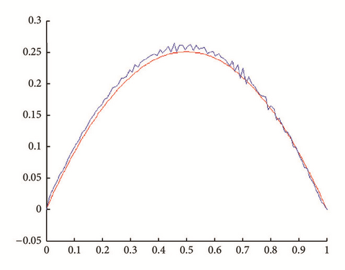
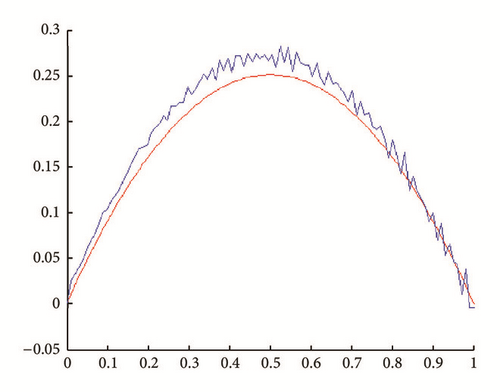
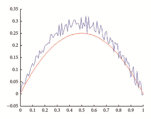
In all figures, the observed function is drawn in red and built function in blue.

Let N be number of points in space and M number of points in time.

6.1.1. The Noncoercive Case

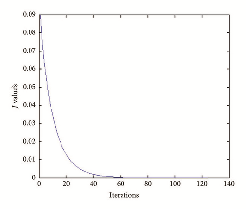
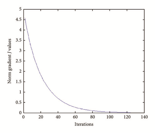
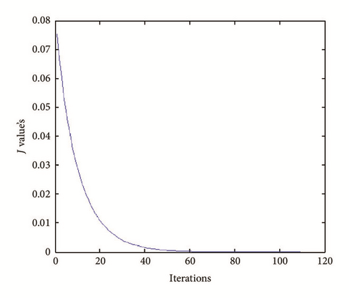
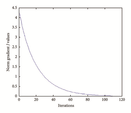
Let α = 1/2, λ = 0 and parameters N = 100, M = 100.

(i) Tests with err = 0. See Figures 1, 2, 3, and 4.

Details are in the caption following the image — **Figure 1**
Open in figure viewer PowerPoint

Initial temperature. This figure shows that we can rebuild the initial state.

(ii) Tests with err ≠ 0. In Figures 5, 6, 7, and 8, is drawn in red and ψ₀ (rebuilt initial condition) in blue.

6.1.2. Sub Critical Potential Case

Let α = 1/2, λ = −(1 − α)²/4, β = 3/4 and the parameters N = 100, M = 100.

(i) Tests with err = 0. See Figures 9, 10, 11, and 12.

(ii) Tests with err ≠ 0. See Figures 13, 14, 15, and 16.

6.2. Hybrid Algorithm

The genetic algorithms (GA) are adaptive search and optimization methods that are based on the genetic processes of biological organisms. Their principles have been first laid down by Holland. The aim of GA is to optimize a problem-defined function, called the fitness function. To do this, GA maintain a population of individuals (suitably represented candidate solutions) and evolve this population over time. At each iteration, called generation, the new population is created by the process of selecting individuals according to their level of fitness in the problem domain and breeding them together using operators borrowed from natural genetics, as, for instance, crossover and mutation. As the population evolves, the individuals in general tend toward the optimal solution [21–24]. The basic structure of a GA is the following:

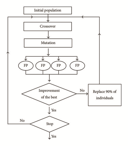
(1) Initialize a population of individuals;
(2) Evaluate each individual in the population;
(3) While the stop criterion is not reached do
{
(4) Select individuals for the next population;
(5) Apply genetic operators (crossover, mutation) to produce new individuals;
(6) Evaluate the new individuals;
}
(7) return the best individual.

The hybrid methods combine principles from genetic algorithms and other optimization methods. In this approach, we will combine the genetic algorithm with method descent (steepest descent algorithm (FP)).

We assume that we have a partial knowledge of background state ψ^b at certain points (x_i) _i∈I, I ⊂ {1,2, …, N + 1}.

We assume the individual is a vector ψ₀; the population is a set of individuals.

The initialization of individual is as follows:

()

Starting by initial population, we apply genetic operators (crossover, mutation) to produce a new population in which each individual is an initial point for the descent method (FP). When a specific number of generations is reached without improvement of the best individual, only the fittest individuals (e.g., the first 10% fittest individuals in the population) survive. The remaining die and their place is occupied by new individuals with new genetic (45% are chosen randomly; the other 45% are chosen as (96)). At each generation we keep the best. The algorithm ends when |J(ψ₀)| < μ or generation⩾Maxgen, where μ is a given precision (see Figure 17).

The main steps for descent method (FP) at each iteration are the following:

(i)
Calculate ψ^k solution of (6) with initial condition ψ₀.
(ii)
Calculate P^k solution of (76).
(iii)
Calculate the descent direction d_k = −∇J(ψ₀).
(iv)
Find t_k = argmin_t>0⁡J(ψ₀ + td_k).
(v)
Update the variable ψ₀ = ψ₀ + t_kd_k.

The algorithm ends when |J(ψ₀)| < μ, where μ is a given small precision.

t_k is chosen by the inaccurate linear search by Rule Armijo-Goldstein as follows:

let α_i, β ∈ [0,1[ and α > 0.
if
t_k = α_i and stop
if not
α_i = αα_i.

Consider we know 20% of values of background state (ψ^b), in this test we try to build the solution with the hybrid method.

In the figures below, the observed function is drawn in red and built function in blue.

Let N be number of points in space and M number of points in time.

6.2.1. The Noncoercive Case

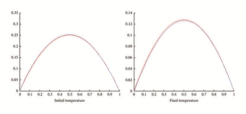
Let α = 1/2, λ = 0 and parameters N = 100, M = 100, number of individuals = 30, and number of generations = 2000.

The test with simple descent gives Figure 18.

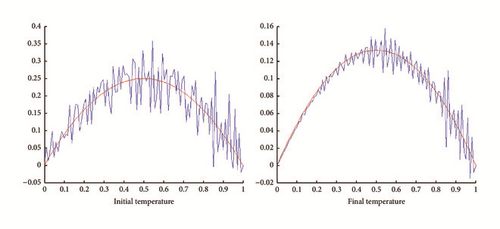
The test with genetic algorithm gives Figure 19.

Now we turn the hybrid algorithm. This gives Figure 20.

6.2.2. Subcritical Potential Case

Let α = 1/2, λ = −(1 − α)²/4, β = 3/4 and parameters N = 100, M = 100, number of individuals = 30, and number of generations = 2000.

The test with simple descent gives Figure 21.

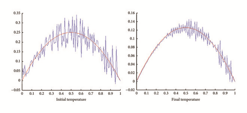
The test with genetic algorithm gives Figure 22.

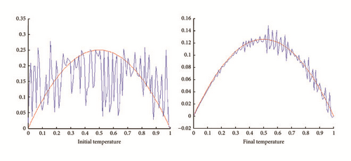
Now we turn the hybrid algorithm. This gives Figure 23.

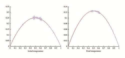
6.3. Comparison between Hybrid Approach and Tikhonov Approach

Here, we assume that we know 20% of values of background state (ψ^b).

(i) Noncoercive Case. see Tables 1 and 2.

Table 1. Results on the Tikhonov approach. Comparison between different values of regularizing coefficient ε. The smallest value of J is reached when ε = 10⁻⁰⁶.

ε	Minimum value of J	Elapsed time (seconds)
10⁻⁰⁸	1.106317 · 10⁻⁰²	8.38
10⁻⁰⁷	1.092014 · 10⁻⁰²	24.47
10⁻⁰⁶	6.630517 · 10⁻⁰³	23.11
10⁻⁰⁵	7.752620 · 10⁻⁰³	21.50
10⁻⁰⁴	7.857129 · 10⁻⁰³	22.64
10⁻⁰³	8.510799 · 10⁻⁰³	18.95
10⁻⁰²	8.733989 · 10⁻⁰³	15.01
10⁻⁰¹	1.018406 · 10⁻⁰²	17.33
1	1.552344 · 10⁻⁰²	6.04

Table 2. Results on the hybrid method.

Minimum value of J	Elapsed time
6.581908 · 10⁻⁰³	1 min
5.850810 · 10⁻⁰³	2 min
3.362100 · 10⁻⁰⁴	7 min
1.071378 · 10⁻⁰⁴	11 min
8.739839 · 10⁻⁰⁵	23 min
5.958016 · 10⁻⁰⁵	6 h 43 min
6.175260 · 10⁻⁰⁶	11 h 20 min

The minimum value of J reached by the Tikhonov algorithm was 6.630517 · 10⁻⁰³, whereas with the hybrid algorithm it was possible to reach the value 6.175260 · 10⁻⁰⁶ in 11 h and 20 min with knowledge of 20% of ψ^b; if we take more than 20%, we got less than elapsed time.

(ii) Subcritical Potential Case. see Tables 3 and 4.

Table 3. Results on the Tikhonov aporoach. Comparison between different values of regularizing coefficient ε. The smallest value of J is reached when ε = 10⁻⁰³.

ε	Minimum value of J	Elapsed time (seconds)
10⁻⁰⁸	1.113538 · 10⁻⁰²	10.91
10⁻⁰⁷	1.188092 · 10⁻⁰²	8.68
10⁻⁰⁶	1.099187 · 10⁻⁰²	8.75
10⁻⁰⁵	1.267204 · 10⁻⁰²	7.91
10⁻⁰⁴	9.648060 · 10⁻⁰³	11.17
10⁻⁰³	7.320995 · 10⁻⁰³	11.61
10⁻⁰²	9.188603 · 10⁻⁰³	10.20
10⁻⁰¹	9.799159 · 10⁻⁰³	9.57
1	1.042463 · 10⁻⁰²	9.66

Table 4. Results on the hybrid method.

Minimum value of J	Elapsed time
7.605018 · 10⁻⁰³	1 min
7.505279 · 10⁻⁰³	2 min
1.762564 · 10⁻⁰³	4 min
9.407809 · 10⁻⁰⁴	43 min
2.981666 · 10⁻⁰⁵	1 h 56 min
1.378356 · 10⁻⁰⁵	6 h 43 min
8.203546 · 10⁻⁰⁶	13 h 40 min

The minimum value of J reached by the Tikhonov algorithm was 7.320995 · 10⁻⁰³, whereas with the hybrid algorithm it was possible to reach the value 8.203546 · 10⁻⁰⁶ in 13 h and 40 min with knowledge of 20% of ψ^b; if we take more than 20%, we got less than elapsed time.

7. Conclusion

In this paper, we have presented the regularization method and the hybrid method which are applied to determine an initial state from the point of measurements of parabolic degenerate/singular problem. These methods have proven efficiency to rebuild the solution. The proposed reconstruction algorithms are easily implanted.

The elapsed time of the hybrid method is long enough. To reduce it, in our coming work we will use the multiprogramming to run two approaches of parallelism.

Conflicts of Interest

The authors declare that there are no conflicts of interest regarding the publication of this paper.

References

1 Isakov V., Inverse Problems for Partial Differential Equations, 1998, Springer, New York, NY, USA, https://doi.org/10.1007/978-1-4899-0030-2, MR1482521.
10.1007/978-1-4899-0030-2
Google Scholar
2 Kirsch A., An Introduction to the Mathematical Theory of Inverse Problems, 1999, Springer, New York, NY, USA, https://doi.org/10.1007/978-1-4419-8474-6, MR3025302.
Google Scholar
3 Buchot J.-M. and Raymond J.-P., A linearized model for boundary layer equations, Optimal control of complex structures (Oberwolfach, 2000), Internat. Ser. Numer. Math, 2002, 139, Birkhäuser, Basel, Swizerland, 31–42, MR1901628.
Google Scholar
4 Beauchard K. and Zuazua E., Some controllability results for the 2D Kolmogorov equation, Annales de l′Institut Henri Poincare (C) Non Linear Analysis. (2009) 26, no. 5, 1793–1815, https://doi.org/10.1016/j.anihpc.2008.12.005, MR2566710.
10.1016/j.anihpc.2008.12.005
Web of Science® Google Scholar
5 Shimakura N., Partial differential operators of elliptic type, 1992, 99, American Mathematical Society, Providence, RI, USA, Translations of Mathematical Monographs, MR1168472.
10.1090/mmono/099
Google Scholar
6 Fleming W. H. and Viot M., Some measure-valued Markov processes in population genetics theory, Indiana University Mathematics Journal. (1979) 28, no. 5, 817–843, https://doi.org/10.1512/iumj.1979.28.28058, MR542340, Zbl0444.60064.
10.1512/iumj.1979.28.28058
Web of Science® Google Scholar
7 Emamirad H., Goldstein G. R., and Goldstein J. A., Chaotic solution for the Black-Scholes equation, Proceedings of the American Mathematical Society. (2012) 140, no. 6, 2043–2052, https://doi.org/10.1090/S0002-9939-2011-11069-4, MR2888192.
10.1090/S0002-9939-2011-11069-4
Web of Science® Google Scholar
8 Fragnelli G. and Mugnai D., Carleman estimates for singular parabolic equations with interior degeneracy and non smooth coefficients, Advances in Nonlinear Analysis. (2016) https://doi.org/10.1515/anona-2015-0163, MR3498150.
10.1515/anona-2015-0163
Web of Science® Google Scholar
9 Bourquin F. and Nassiopoulos A., Assimilation thermique 1D par méthode adjointe libérée, Problèmes Inverses, 2006, Collection Recherche du LCPC.
Google Scholar
10 Min T., Geng B., and Ren J., Inverse estimation of the initial condition for the heat equation, International Journal of Pure and Applied Mathematics. (2013) 82, no. 4, 581–593, 2-s2.0-84874033700, https://doi.org/10.12732/ijpam.v82i4.7.
10.12732/ijpam.v82i4.7
Google Scholar
11 Santos L. B. L., Chiwiacowsky L. D., and Campos-Velho H. F., Genetic algorithm and variational method to identify initial conditions: worked example in hyperbolic heat transfer, TEMA. Tendências em Matemática Aplicada e Computacional. (2013) 14, no. 2, 265–276, MR3162055.
Google Scholar
12 Bonnet M., Ecole Centrale de Paris Mention Matière, Structures, Fluides, Rayonnement Spécialité Dynamique des Structures et Systèmes Couplés [M.S. thesis], 2008, [email protected].
Google Scholar
13 Jens F., Generalized Tikhonov regularization, Basic theory and comprehensive results on convergence rates [Dissertation], 2011, Fakultät für Mathematik Technische Universität Chemnitz, Chemnitz.
Google Scholar
14 Alabau-Boussouira F., Cannarsa P., and Fragnelli G., Carleman estimates for degenerate parabolic operators with applications to null controllability, Journal of Evolution Equations. (2006) 6, no. 2, 161–204, https://doi.org/10.1007/s00028-006-0222-6, MR2227693, Zbl1103.35052, 2-s2.0-33744475607.
10.1007/s00028-006-0222-6
Web of Science® Google Scholar
15 Ait Ben Hassi E. M., Ammar Khodja F., Hajjaj A., and Maniar L., Carleman estimates and null controllability of coupled degenerate systems, Evolution Equations and Control Theory. (2013) 2, no. 3, 441–459, https://doi.org/10.3934/eect.2013.2.441, MR3093224, Zbl1272.35124, 2-s2.0-84903604586.
10.3934/eect.2013.2.441
Web of Science® Google Scholar
16 Cannarsa P. and Fragnelli G., Null controllability of semilinear degenerate parabolic equations in bounded domains, Electronic Journal of Differential Equations. (2006) 136, 1–20, MR2276561.
Google Scholar
17 Cannarsa P., Martinez P., and Vancostenoble J., Carleman estimates for a class of degenerate parabolic operators, SIAM Journal on Control and Optimization. (2008) 47, no. 1, article no. 119, https://doi.org/10.1137/04062062X, MR2373460.
10.1137/04062062X
Web of Science® Google Scholar
18 Cannarsa P., Martinez P., and Vancostenoble J., Null controllability of degenerate heat equations, Advances in Differential Equations. (2005) 10, no. 2, 153–190, MR2106129, Zbl1145.35408, 2-s2.0-33744486668.
10.57262/ade/1355867887
Web of Science® Google Scholar
19 Vancostenoble J., Improved Hardy-Poincaré inequalities and sharp Carleman estimates for degenerate/singular parabolic problems, Discrete and Continuous Dynamical Systems. (2011) 4, no. 3, 761790, https://doi.org/10.3934/dcdss.2011.4.761, MR2746432.
10.3934/dcdss.2011.4.761
Web of Science® Google Scholar
20 Ait Ben Hassi E. M., Ammar Khodja F., Hajjaj A., and Maniar L., Null controllability of degenerate cascade systems, Journal of Evolution Equations and Control Theory. (2013) 2, no. 3, 441–459, MR3093224.
10.3934/eect.2013.2.441
Web of Science® Google Scholar
21 Michalewicz Z., Genetic Algorithms + Data Structures = Evolution Programs, 1996, Springer, New York, NY, USA, https://doi.org/10.1007/978-3-662-07418-3, MR1329091, Zbl0818.68017.
10.1007/978-3-662-03315-9
Web of Science® Google Scholar
22 Goldberg D. E., Genetic Algorithms in Search, Optimisation and Machine Learning, 1989.
Google Scholar
23 Holland J. H., Adaptation in Natural and Artificial Systems, 1975, University of Michigan Press, Oxford, UK, MR0441393.
Google Scholar
24 Koza J. R., Genetic Programming, 1992, MIT Press.
Google Scholar

Citing Literature

All articles

Identifying Initial Condition in Degenerate Parabolic Equation with Singular Potential

Abstract

1. Introduction

2. Problem Statement and Main Result

3. Proof

4. Gradient of J

5. Discretization of Problem