The determinant of a matrix is very powerful tool that helps in establishing properties of matrices. Indisputably, its importance in various engineering and applied science problems has made it a mathematical area of increasing significance. From developed and existing methods of finding determinant of a matrix, basketweave method/Sarrus’ rule has been shown to be the simplest, easiest, very fast, accurate, and straightforward method for the computation of the determinant of 3 × 3 matrices. However, its gross limitation is that this method/rule does not work for matrices larger than 3 × 3 and this fact is well established in literatures. Therefore, the state-of-the-art methods for finding the determinants of 4 × 4 matrix and larger matrices are predominantly founded on non-basketweave method/non-Sarrus’ rule. In this work, extension of the simple, easy, accurate, and straightforward approach to the determinant of larger matrices is presented. The paper presents the developments of new method with different schemes based on the basketweave method/Sarrus’ rule for the computation of the determinant of 4 × 4. The potency of the new method is revealed in generalization of the basketweave method/non-Sarrus’ rule for the computation of the determinant of n × n (n > 3) matrices. The new method is very efficient, very consistence for handy calculations, highly accurate, and fastest compared to other existing methods.

1. Introduction

Over the years, the subject, linear algebra has been shown to be the most fundamental component in mathematics as it presents powerful tools in wide varieties of areas from theoretical science to engineering, including computer science. Its important role and abilities in solving real life problems and in data clarification [1] have led it to be frequently applied in all the branches of science, engineering, social science, and management. During the applications and analysis in such areas of studies, a system of linear equations can be written in matrix form and solving the system of linear equations and the inversion of matrices is necessary which is mainly dependent on determinant (a real number or a function of the elements of an n × n matrix that yields a single number that well determines something about the matrix). Therefore, the importance of finding the determinant in linear algebra cannot be overemphasized as it does not only help in finding solution to systems of linear equations but it also helps determine whether the system has a unique solution and helps establish relationship and properties of matrices. Undoubtedly, the computation of such single number called the determinant is fundamental in linear algebra. It is one of the basic concepts in linear algebra which has major applications in various branches of engineering and applied science problems such as in the solutions systems of linear equations and also in finding the inverse of an invertible matrix. Also, many complicated expressions of electrical and mechanical systems can be conveniently handled by expressing them in “determinant form.” Therefore, it has become a mathematical area of increasing significance as the computation of the determinant of an n × n matrix A of numbers or polynomials is a classical problem and challenge for both numerical and symbolic methods. Consequently, various direct and nondirect methods such as butterfly method, Sarrus’ rule, triangle’s rule, Gaussian elimination procedure, permutation expansion or expansion by the elements of whatever row or column, pivotal or Chio’s condensation method, Dodgson’s condensation method, LU decomposition method, QR decomposition method, Cholesky decomposition method, Hajrizaj’s method, and Salihu and Gjonbalaj’s method [1–35] have been proposed for finding the determinant of n × n matrices. In the gamut of the methods or rules for finding the determinant of the n × n matrices, Sarrus’ rule (a method of finding the determinant of 3 × 3 matrices named after a French mathematician, Pierre Frédéric Sarrus (1798–1861)) has been shown to be the simplest, easiest, fastest, and very straightforward method. Although the wide range of applications of the rule for the computation of the determinant of 3 × 3 matrices is well established, it is grossly limited in applications since it cannot be used for finding the determinants of 4 × 4 matrices and larger matrices. Moreover, the combined idea of finding determinant of 2 × 2 matrices using butterfly method which is the conventional idea in all literatures and using Sarrus’ rule for finding the determinant of 3 × 3 matrices is termed basketweave method. However, the basketweave method does not work on matrices larger than 3 × 3 [1]. Therefore, for larger matrices, the computations of determinants are carried out by methods such as row reduction or column reduction, Laplace expansion method, Dodgson’s condensation method, Chio’s condensations, triangle’s rule, Gaussian elimination procedure, LU decomposition, QR decomposition, and Cholesky decomposition. However, these methods are not as simple, easy, fast, and very straightforward as basketweave method/Sarrus’ rule. Additionally, the cost of the computation of the determinant of a matrix of order n is about 2n³/3 arithmetic operations using Gauss elimination; if the order n of the matrix is large enough, then the computation is not feasible. Therefore, Rezaifar and Rezaee [1] developed a recursion technique to evaluate the determinant of a matrix. In their quests for establishing a new scheme for the generalization of Rezaifar and Rezaee’s procedure, Dutta and Pal [36] pointed out the limitation of Rezaifar and Rezaee’s procedure as it fails to evaluate the values of the determinants of matrices in some cases. Therefore, in this paper, a new method using different schemes based on Sarrus’ rule was developed to carry out the computation of the determinant of 4 × 4 matrices. The developed method is shown to be very quick, easy, efficient, very usable, and highly accurate. It creates opportunities to find other new methods based on Sarrus’ rule to compute determinants of higher orders. Also, the new approach has been shown to be applicable to the computation of determinants of larger matrices such as 5 × 5, 6 × 6, and all other n × n (n > 6) matrices.

2. Definition of Determinants

The determinant of n × n matrix square matrix A = [a_ij] is a real number or a function of the elements of the matrix which well determines something about the matrix. It determines whether the system has a unique solution and whether the matrix is singular or not.

The determinant of an n-order matrix will be called sum, which has n! different terms which will be formed of matrix A elements.

Let A be an n × n matrix:

()

Then determinant of A is

()

where

()

The determinant of matrix A could also be written in Laplace cofactor form as

()

3. Existing Methods of Computation of Determinants

The easiest way to find the determinant of a matrix is to use a computer program which has been optimized so as to reduce the computational time and cost, but there are several ways to do it by hand [37–43]. Therefore, the computation of determinants of matrices has been carried out by some existing methods in literature such as basketweave method, butterfly method, Sarrus’ method, triangle’s rule, Gaussian elimination procedure, permutation expansion or Laplace expansion by the elements of whatever row or column, row reduction method, column reduction method, pivotal or Chio’s condensation method, Dodgson’s condensation method, LU decomposition method, QR decomposition method, Cholesky decomposition method, Hajrizaj’s method, Salihu and Gjonbalaj’s method, Rezaifar and Rezaee’s method, and Dutta and Pal’s method. The simplest among these methods is the basketweave method which could be stated as the combination of butterfly method for determinant computation of 2 × 2 matrices and Sarrus’ rule for determinant computation of 3 × 3 matrices.

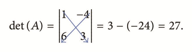
3.1. The Butterfly Method

A 2 × 2 matrix is written as

()

In order to find the determinant of the 2 × 2 matrix, we carry out the diagonal products. We then subtract the diagonal product as we go right to left from the diagonal product of a square matrix as left to right as follows:

()

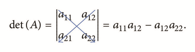
Example 1. Evaluate :

()

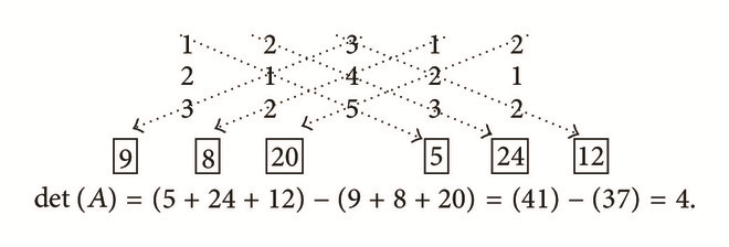
3.2. Sarrus’ Method

A 3 × 3 matrix is written as

()

Sarrus’ rule which is sometimes also called the basketweave method is an alternative way to evaluate the determinant of a 3 × 3 matrix. It is a method that is only applicable to 3 × 3 matrices. It follows the same process as carried out in the 3 × 3 matrix, except that we need to repeat the first two columns to the right of the original matrix and then do the basketweave method. Therefore, a 3 × 5 array is constructed by writing down the entries of the 3 × 3 matrix and then repeating the first two columns at the back of the third column. We calculate the products along the six diagonal lines shown in the diagram. The determinant is equal to the sum of products along diagonals labeled 1, 2, and 3 minus the sum of the products along the diagonals labeled 4, 5, and 6. An example is shown as follows:

()

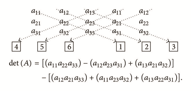
Example 2. Evaluate :

()

Multiplication of the numbers on the same line, addition of the ones from down-going lines, and subtraction of the ones from up-going lines are an approach that led to the name “the basketweave method.” Unfortunately, the simple weave method does not work on matrices larger than 3 × 3.

The use of Laplace cofactor expansion along either the row or column is a common method for the computation of the determinant of 3 × 3, 4 × 4, and 5 × 5 matrices. The evaluation of the determinant of an n × n matrix using the definition involves the summation of n! terms, with each term being a product of n factors. As n increases, this computation becomes too cumbersome. This drawback is not only peculiar to Laplace cofactor expansion method as other common methods developed in literatures also required additional computational cost and time for the computation of determinant. Therefore, in recent times, different techniques have been devised in literatures. However, these techniques are not as simple, easy, fast, and very straightforward as the basketweave method/Sarrus’ rule. Additionally, many of them come with relatively high computational cost and time.

4. The Development of the New Methods for the Computation of Determinants

Consider a 4 × 4 matrix whose determinant is required, given as follows:

()

Following the definition given in Section 2, the conventional method of finding the determinant by Laplace cofactor expansion method is carried out as follows.

Expanding along the first row, we have

()

Again, expanding each of the 3 × 3 matrices along the first row, we have

()

Now, we have

()

So, it is shown that 4! different terms will be needed to compute the determinant of the forth-order matrices.

In order to generate these 4! different terms (24 terms), we have the following 3 different 4 × 4 matrices as follows:

()

In the arrangements, C1, C2, C3, and C4 represent the first, the second, the third, and the fourth columns, respectively, as given in the original 4 × 4 matrix. We could see in (15) that the first arrangement

of 4 × 4 matrix remains the same as given in the original matrix A. To get the second arrangement

of another 4 × 4 matrix, remove and transfer the second column in the first arrangement to the last column of the given 4 × 4 matrix A. To get the third arrangement

of another new 4 × 4 matrix, remove and transfer the second column in the second arrangement to be the last column of the second 4 × 4 matrix. This forms the third 4 × 4 matrix. After the third step, we need not go further to perform the procedure of removing and transferring the second column in the first arrangement to the last column of the given 4 × 4 matrix because if we do we will end up repeating the first step or getting the first original 4 × 4 matrix in this procedure. In fact, this approach helps us know when to stop the procedures. That is why the last arrangement was cancelled.

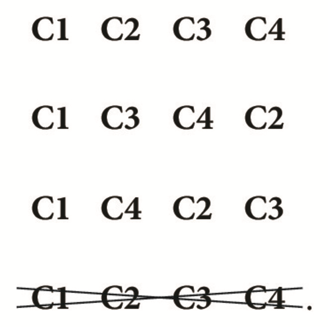
Following the procedure, we have 4 × 4 matrices.

The first 4 × 4 matrix is

()

The second 4 × 4 matrix is

()

The third 4 × 4 matrix is

()

From the above, 10 new schemes based on Sarrus’ rule were developed for the computation of the determinant of the 4 × 4 matrix.

In the new method/scheme, the next step to find det⁡(A) after the arrangements is as follows:

(1)
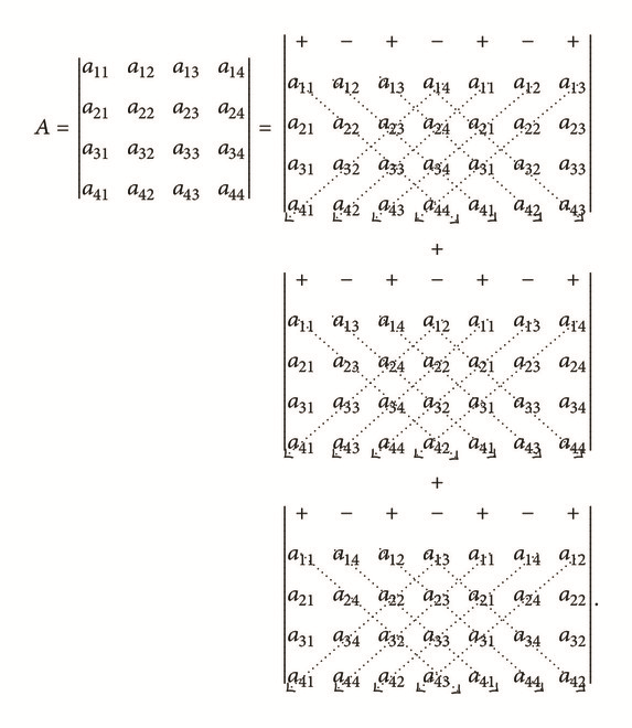
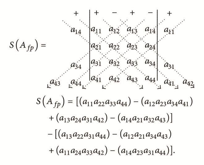
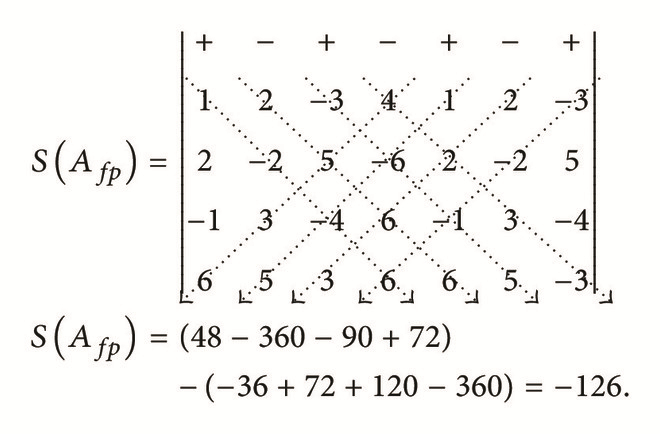
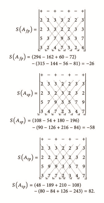
In the first submatrix A_fp, rewrite the 1st, 2nd, and 3rd columns on the right-hand side of matrix A_fp (as columns 5, 6, and 7). To the resulting 4 × 7 augmented matrix, assign “+” to the leading element in the odd numbered columns and assign “−” sign to the leading element in the even numbered columns. This gives
()
This is the first part of the solution of the computation of determinant of the given 4 × 4 matrix.
(2)
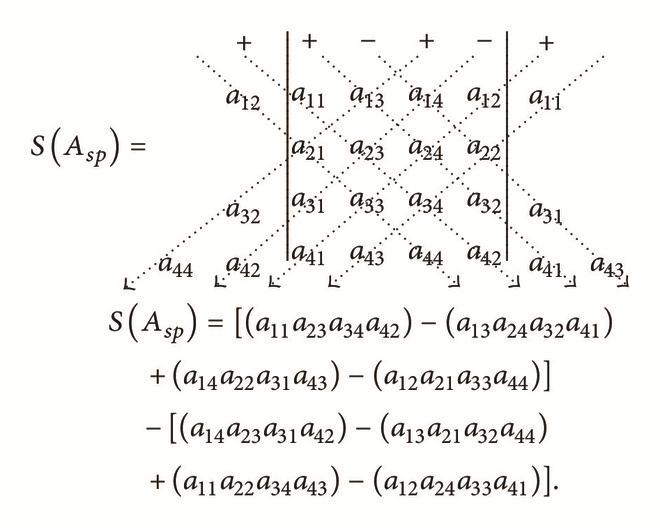
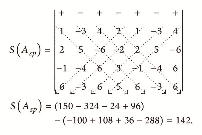
In the second submatrix A_sp, rewrite the 1st, 2nd, and 3rd columns on the right-hand side of matrix A_sp ( as columns 5, 6, and 7). As in the first step, to the augmented matrix, assign “+” to the leading element in the odd numbered columns and assign “−” sign to the leading element in the even numbered columns and then apply Sarrus’ rule.
()
This is the second part of the computation of determinant of the given 4 × 4 matrix.
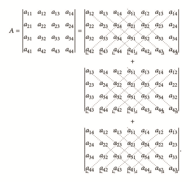
(3)
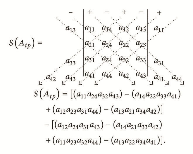
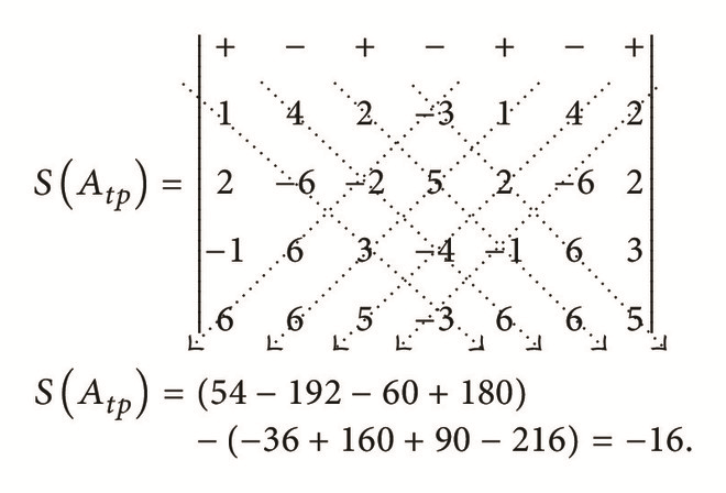
In the third submatrix A_tp, rewrite the newest 1st, 2nd, and 3rd columns on the right-hand side of matrix A_tp (as columns 5, 6, and 7). And again, to the augmented matrix, assign “+” to the leading element in the odd numbered columns and assign “−” sign to the leading element in the even numbered columns and then apply Sarrus’ rule.
()
This is the third part of the computation of determinant of the given 4 × 4 matrix.
(4)
For each of augmented matrices A_argfp, A_argsp, and A_argtp, apply Sarrus’ rule by adding the products along the four full diagonals that extend from upper left to lower right and subtract the products along the four full diagonals that extend from the lower left to the upper right. After finding the determinant of the augmented matrices A_argfp, A_argsp, and A_argtp, the addition of the results after applying Sarrus’ rule on the augmented matrices A_argfp, A_argsp, and A_argtp is the determinant of A. This is shown as follows:

()

Therefore, we have (9) which is equivalent in all entireties to (14) when Laplace cofactor expansion method is used:

()

Alternatively, the new scheme could be carried out in another way. In the alternative way, the algorithm still remains the same but the difference is in the manner where the submatrices A_fp, A_sp, and A_tp are constructed. In this scheme, we rewrite the 1st, 2nd, and 3rd columns on the left-hand side of matrix A (as columns 0, −1, and −2) to form the required 4 × 7 augmented matrix. Therefore, we have the submatrices A_fp, A_sp, and A_tp given as

()

As before,

()

Again, we arrived at (14):

()

Furthermore, the new scheme could be carried out in another way. In this alternative approach to the new method, the submatrices A_fp, A_sp, and A_tp are constructed via a different approach. The determinant of the given fourth-order matrix A is found as shown below.

First submatrix is

()

Second submatrix is

()

Third submatrix is

()

As before,

()

Then, we arrived at (14):

()

5. Numerical Examples

In our numerical example, we investigate the workability, correctness, and efficiency of the use of the new method. We do this by first applying the other known and common methods such as expansion of cofactors method, pivotal condensation method, and the new method based on Sarrus’ rule.

Example 1. One has

()

Using Laplace Expansion of Cofactor Method. One has

()

Using Chio’s Pivotal Condensation Method. One has

()

Initialize D = 1 and reduce A to row echelon form [35]:

()

Adding −2 times the first row to the second row, D remains 1:

()

Adding 1 times the first row to the third row, D remains 1:

()

Adding −6 times the first row to the fourth row, D remains 1:

()

Multiplying the second row by −1/6, D ← D(−6) = 1(−6) = −6:

()

Adding −5 times the second row to the third row, D remains −6:

()

Adding 7 times the second row to the fourth row, D remains −6.

Multiplying the second row by 6/13, D ← D(13/6) = −6(13/6) = −13:

()

Adding −13/6 times the third row to the fourth row, D remains −13:

()

The matrix is now in row echelon form with diagonal elements 1, 1, 1, and 0.

Thus, det⁡A = −13(1)(1)(0) = 0.

Using the New Method (Gbemi’s Method). One has

()

Hence,

()

Applying Sarrus’ rule to the second part A_sp,

()

Applying Sarrus’ rule to the third part A_tp,

()

Therefore,

()

Example 2. ⁡

Using the Laplace Expansion of Cofactors Method. One has

()

Using the New Method (Gbemi’s Method). One has

()

Hence,

()

Therefore,

()

Hence,

()

It should not be that we only apply the first scheme in this example. If we use any of the 10 schemes developed in work, we will still arrive at the same results.

6. Efficiency of the New Method

6.1. Asymptotic Analysis

In order to determine the efficiency of the method, an asymptotic analysis was carried out using big-O. The advantage of asymptotic analysis is that it is independent of the computer specifications. This will be used to compare the existing methods with the new method.

The conventional method in most texts and literatures is the Laplace expansion method which evaluates the determinant as a weighted sum of its submatrices. It is well established in literature that the run time of the Laplace expansion method for finding determinant is O(n!).

6.1.1. Run Time of New Method

The new method evaluates the determinant of a 4 × 4 matrix as an extension of Sarrus’ rule. Thus, for every diagonal, there are n items that are visited. Thus, the running time is O(n²). This can also be verified from the MATLAB program. There are two nested for loops which means an O(n²) algorithm.

6.1.2. Run Time of Other Variations of the New Method

Analyzing the other variations of the new method, the run time is O(n²).

7. Programming

This section presents the evaluation of the new approach (called the G-method) and its ability to be used in programming (i.e., as a subroutine for more applications); the program is written in MATLAB. Also, the MATLAB codes for Rezaifar and Rezaee [1] and Laplace expansion method are also presented as shown in Algorithm 1.

Algorithm 1

function answer = GMethod(A,part)
%% Developed by Sobamowo M. Gbeminiyi************************************
%% GMethod stands for Gbeminiyi’s method.
n = length(A);
sum1 = 0;
sum2 = 0;
for i = 1:1:n
sum3 = 1;
sum4 = 1;
for j = 1:1:n
sum3 = sum3*A(j,non_zero(mod(i+j-1,4),4));
sum4 = sum4*A(n - j + 1,non_zero(mod(i+j-1,4),4));
end
sum1 = sum1 + ((-1) ^∧(i+1))*sum3;
sum2 = sum2 + ((-1) ^∧(i))*sum4;
end
answer = (sum1 - sum2);
if part <= 2
answer = answer + GMethod([A(:,1),A(:,3:n),A(:,2)],part+1);
end
end
function answer = RMethod(m)
%% Developed by Omid Rezaifar.****************************************
%% RMethod stands for Rezaifar Method.
%% Developed by Omind Rezaifar.
%% This code was extracted from [31, 38–42]
n = length(m);
if n == 1
answer = m;
elseif n == 2
answer = m(1,1)*m(2,2) - m(1,2)*m(2,1);
else
m11 = m(2:n,2:n);
m1n = m(2:n,1:n -1);
mn1 = m(1:n -1,2:n);
mnn = m(1:n - 1, 1:n -1);
m11nn = m11(1:n -2, 1:n-2);
answer = RMethod(m11)*RMethod(mnn) - RMethod(m1n)*RMethod(mn1);
answer = answer / RMethod(m11nn);
end
end
function [answer] = ExpansionMethod(A)
%% Laplace Expansion Method ******************************************
%%
n = length(A);
if n==1
answer = A;
else
if n == 2
answer = A(1,1)*A(2,2) - A(1,2)*A(2,1);
else
answer = 0;
for i = 1:1:n
answer = answer + ((-1) ^∧(1+i)*A(1,i))*ExpansionMethod([A(2:n,1:i - 1), A(2:n, i+1:n)]);
end
end
end
>> ExecutionTest1
∗∗∗∗∗∗∗∗∗∗∗∗∗∗∗∗∗∗∗∗
Matrix Executed
∗∗∗∗∗∗∗∗∗∗∗∗∗∗∗∗∗∗∗∗
∗∗∗∗∗∗∗∗Average Time per Execution For Laplace Expansion Method∗∗∗∗∗∗∗∗∗
Number of Executions = 1000
Total Time for Execution = 0.453
Average Time per Execution = 0.000453
∗∗∗∗∗∗∗∗∗∗∗∗∗∗∗∗∗∗∗∗
>> ExecutionTest2
∗∗∗∗∗∗∗∗∗∗∗∗∗∗∗∗∗∗∗∗
Matrix Executed
∗∗∗∗∗∗∗∗∗∗∗∗∗∗∗∗∗∗∗∗
∗∗∗∗∗∗∗∗Average Time per Execution For Gbeminiyi Method (G-Method)∗∗∗∗∗∗∗∗∗∗∗
Number of Executions = 1000
Total Time for Execution = 0.218
Average Time per Execution = 0.000218
∗∗∗∗∗∗∗∗∗∗∗∗∗∗∗∗∗∗∗∗
>> ExecutionTest3
∗∗∗∗∗∗∗∗∗∗∗∗∗∗∗∗∗∗∗∗
Matrix Executed
∗∗∗∗∗∗∗∗∗∗∗∗∗∗∗∗∗∗∗∗
∗∗∗∗∗∗∗∗Average Time per Execution For Rezaifar Method∗∗∗∗∗∗∗∗∗
Number of Executions = 1000
Total Time for Execution = 0.359
Average Time per Execution = 0.000359
∗∗∗∗∗∗∗∗∗∗∗∗∗∗∗∗∗∗∗∗

8. Comparison with Existing Methods

The running time O(n²) is far better than O(n!) running time. This means that the G-method (the new method) is more efficient than the existing Laplace expansion method and other existing methods for the computation of 4 × 4 matrix. This fact was also illustrated with the execution time of the MATLAB code run on an Intel® Core™2 Duo CPU 2.00 GHz 4.00 GB (RAM) system. The codes for the Laplace expansion method and G-method were run with a test matrix.

In order to see the difference in execution time and speed of execution more efficiently, the algorithm has to be run many times. Therefore, the codes were run 1000 and 10,000 times on the same matrix, and the average execution time per problem is calculated. The results are shown in Tables 1 and 2.

Table 1. Comparison of time consumption among different methods.

	Laplace expansion method	Rezaifar method	The new method (Gbemi’s method)
Number of executions	1,000	1,000	1,000
Total time for executions	0.453 s	0.359 s	0.218 s
Average time per execution	0.00453 s	0.00359 s	0.00218 s

Table 2. Comparison of time consumption among different methods.

	Laplace expansion method	Rezaifar method	The new method (Gbemi’s method)
Number of executions	10,000	10, 000	10,000
Total time for executions	4.197 s	3.496 s	1.766 s
Average time per execution	0.0004197 s	0.003496 s	0.0001766 s

It can been seen from Tables 1 and 2 that the new method saves much time and the speed of running is faster than the Laplace expansion and Rezaifar’s methods. Although the recursive loops in Rezaifar’s method make it be used more in programming, if the division by zero appears during the computation of the determinant of a matrix, then the method fails to evaluate the value of the determinant unless rows are changed and as a result the determinant altered [1]. This shortcoming or limitation of Rezaifar’s method was also pointed out by Dutta and Pal [36]. However, the newly developed method (G-method) overcomes the limitation of Rezaifar’s method.

For the optimized MATLAB in-built method, for the 1000 number of executions, the total time for execution is 0.015 sec, while the average time per execution is 0.000015 sec. However, it has been pointed out that, commonly in machine programs which required some algorithm to find the determinant of matrices, Gaussian elimination or Gauss-Jordan method is used. This method is based on linear and unilateral approach to find the determinant [1]. It is hoped that if this newly developed algorithm is optimized, it will run faster than the MATLAB in-built method.

9. Conclusion and Future Works

In this paper, efficient techniques based on Sarrus’ rule for computation of the determinant of 4 × 4 matrices have been proposed. The techniques are shown to be very quick, easy, efficient, very usable, and highly accurate. The new method creates opportunities to find other new methods based on Sarrus’ rule to compute determinants of higher orders. Also, the new approach has been shown to be applicable to compute the determinants of larger matrices such as 5 × 5, 6 × 6, and all other n × n (n > 6) matrices. This will be presented in the second part of the paper.

Competing Interests

The author declares that there are no competing interests regarding the publication of this paper.

References

1 Rezaifar O. and Rezaee H., A new approach for finding the determinant of matrices, Applied Mathematics and Computation. (2007) 188, no. 2, 1445–1454, https://doi.org/10.1016/j.amc.2006.11.010, MR2335641, 2-s2.0-34248218009.
10.1016/j.amc.2006.11.010
Web of Science® Google Scholar
2 Abbott J., Bronstein J., and Mulders M., S. Dooley, Fast deterministic computation of determinants of dense matrices, Proceedings of the International Symposium on Symbolic and Algebraic Computation (ISSAC ′99), July 1999, Vancouver, Canada, ACM, 197–204, https://doi.org/10.1145/309831.309934.
10.1145/309831.309934
Google Scholar
3 Ahmed A. A. M. and Bondar K. L., Modern method to compute the determinants of matrices of order 3, Journal of Informatics and Mathematical Sciences. (2014) 6, no. 2, 55–60.
Google Scholar
4 Clarkson K. L., Safe and effective determinant evaluation, Proceedings of the 33rd Annual Symposium on Foundations Computer Science, 1992, Pittsburgh, Pa, USA, IEEE Computer Society Technical Committee on Mathematical Foundations of Computing, IEEE Computer Press, The Institute of Electrical and Electronics Engineers, 387–395.
Google Scholar
5 Dingle B. M., Calculating determinants of symbolic and numeric matrices, Texas, 2005.
Google Scholar
6 Dubbs C. and Siegel D., Computing determinants, The College Mathematics Journal. (1987) 18, no. 1, 48–50, https://doi.org/10.2307/2686317.
10.1080/07468342.1987.11973007
Google Scholar
7 Eberly D., The Laplace Expansion Theorem: Computing the Determinants and Inverses of Matrices, 2007, Geometric Tools, LLC, Scottsdale, Ariz, USA.
Google Scholar
8 Gentleman W. M. and Johnson S. C., The evaluation of determinants by expansion by minors and the general problem of substitution, Mathematics of Computation. (1974) 28, no. 26, 543–548, MR0373369.
10.1090/S0025-5718-1974-0373369-7
Web of Science® Google Scholar
9 Salihu A. and Gjonbalaj Q., New method to compute the determinant of a 4x4 matrix, Proceedings of the 3rd International Mathematics Conference on Algebra and Functional Analysis, May 2009, At Elbasan, Albania.
Google Scholar
10 Assen A. and Venkateswara Rao J., A study on the computation of the determinants of a 3 × 3 matrix, International Journal of Science and Research. (2014) 3, no. 6, 912–921.
Google Scholar
11 Chió F., Mémoire sur les Fonctions Connues Sous le Nom de Résultantes ou de Déterminants, 1853, E. Pons, Turin, Italy.
Google Scholar
12 Dodgson C. L., Condensation of determinants, being a new and brief method for computing their arithmetic values, Proceedings of the Royal Society of London A: Mathematical, Physical and Engineering Sciences. (1866) 15, 150–155, https://doi.org/10.1098/rspl.1866.0037.
10.1098/rspl.1866.0037
Google Scholar
13 Dodgson C. L., Elementary Treatise on Determinants with the Applications to Simultaneous Linear Equations and Algebraical Geometry, 1867, MacMillan, London, UK.
Google Scholar
14 El-Mikkawy M. E. A., A fast algorithm for evaluating nth order tri-diagonal determinants, Journal of Computational and Applied Mathematics. (2004) 166, no. 2, 581–584, https://doi.org/10.1016/j.cam.2003.08.044, 2-s2.0-1542740071.
10.1016/j.cam.2003.08.044
Web of Science® Google Scholar
15 Tofen E. K. and Villard G., K. Shirayanagi and K. Yokoyama, On the complexity of computing determinants^∗ (extended abstract), 9, Proceedings of the 5th Asian Symposium on Computer Mathematics (ASCM ′01), 2001, Singapore, World Scientific, 13–27, Lecture Notes Series on Computing.
Google Scholar
16 Gentleman W. M. and Johnson S. C., Analysis of algorithms, a case study: determinants of polynomials, Proceedings of the 5th annual ACM Symposium on Theory of Computing, 1973, ACM Press, 135–141.
Google Scholar
17 Gjonbalaj Q. and Salihu A., Computing the determinants by reducing the orders by four, Applied Mathematics E-Notes. (2010) 10, 151–158, MR2725712.
Google Scholar
18 Hajrizaj D., New method to compute the determinant of 3 × 3 matrix, International Journal of Algebra. (2009) 3, no. 5, 211–219.
Google Scholar
19 Henrion D. and Šebek M., Improved polynomial matrix determinant computation, IEEE Transactions on Circuits and Systems I: Fundamental Theory and Applications. (1999) 46, no. 10, 1307–1308, https://doi.org/10.1109/81.795848, ZBL0968.65026, 2-s2.0-0033204464.
10.1109/81.795848
Google Scholar
20 Ipsen C. F. and Lee D. J., Determinant approximations, Numerical Linear Algebra with Applications, 2005, John Wiley & Sons, New York, NY, USA.
Google Scholar
21 Kaltofen E., P. S. Wang, On computing determinants of matrices without divisions, Proceedings of the International Symposium on Symbolic and Algebraic Computation (ISSAC ′92), 1992, ACM, 342–349, https://doi.org/10.1145/143242.143350.
10.1145/143242.143350
Google Scholar
22 Kaltofen E. and Villard G., Computing the sign or the value of the determinant of an integer matrix, a complexity survey, Journal of Computational and Applied Mathematics. (2001) 162, no. 1, 133–146.
10.1016/j.cam.2003.08.019
Google Scholar
23 Molinari L. G., Determinants of block tridiagonal matrices, Linear Algebra and Its Applications. (2008) 429, no. 8-9, 2221–2226, https://doi.org/10.1016/j.laa.2008.06.015, MR2446654, 2-s2.0-49249134522.
10.1016/j.laa.2008.06.015
Web of Science® Google Scholar
24 Pan V. Y., Computing the determinant and the characteristic polynomial of a matrix via solving linear systems of equations, Information Processing Letters. (1988) 28, no. 2, 71–75, https://doi.org/10.1016/0020-0190(88)90166-4, MR948861, 2-s2.0-0024031591.
10.1016/0020-0190(88)90166-4
Web of Science® Google Scholar
25 Radić M., A generalization of the determinant of a square matrix and some of its applications in geometry, Matematika. 20, 19–36, 1999 (Serbo-Croatian).
Google Scholar
26 Adrian R. and Torrence E., Shuttling up like a telescope′: lewis carroll′s ‘curious’ condensation method for evaluating determinants, College Mathematics Journal. (2007) 38, no. 2.
Google Scholar
27 Teimoori H., Bayat M., Amiri A., and Sarijloo E., A new parallel algorithm for evaluating the determinant of a matrix of order n, Euro Combinatory. (2005) 123–134.
Google Scholar
28 Chen X.-B., A fast algorithm for computing the determinants of banded circulant matrices, Applied Mathematics and Computation. (2014) 229, 201–207, https://doi.org/10.1016/j.amc.2013.12.048, MR3159867, 2-s2.0-84891790894.
10.1016/j.amc.2013.12.048
Web of Science® Google Scholar
29 Goldfinger Y., Determinant by cofactor expansion using the cell processor, CMSC 49lA, 2008.
Google Scholar
30 Bozkurt D. and Tam T.-Y., Determinants and inverses of circulant matrices with Jacobsthal and Jacobsthal-lucas numbers, Applied Mathematics and Computation. (2012) 219, no. 2, 544–551, https://doi.org/10.1016/j.amc.2012.06.039, MR2956985, 2-s2.0-84864997038.
10.1016/j.amc.2012.06.039
Web of Science® Google Scholar
31 Lang S., Undergraduate Algebra, 1990, 2nd edition, Springer, New York, NY, USA.
Google Scholar
32 Sogabe T., A fast numerical algorithm for the determinant of a pentadiagonal matrix, Applied Mathematics and Computation. (2008) 196, no. 2, 835–841, https://doi.org/10.1016/j.amc.2007.07.015, MR2388737, 2-s2.0-38649106820.
10.1016/j.amc.2007.07.015
Web of Science® Google Scholar
33 Lv X.-G., Huang T.-Z., and Le J., A note on computing the inverse and the determinant of a pentadiagonal Toeplitz matrix, Applied Mathematics and Computation. (2008) 206, no. 1, 327–331, https://doi.org/10.1016/j.amc.2008.09.006, MR2474978, 2-s2.0-55949114665.
10.1016/j.amc.2008.09.006
Web of Science® Google Scholar
34 Pan V., Complexity of computations with matrices and polynomials, SIAM Review. (1992) 34, no. 2, 225–262, https://doi.org/10.1137/1034049, MR1166176.
10.1137/1034049
Web of Science® Google Scholar
35 Lipschutz S. and Lipson M., Schaum′s Outlines Linear Algebra, 2004, 3rd edition, McGraw-Hill Companies, New York, NY, USA.
Google Scholar
36 Dutta J. and Pal S. C., Generalization of a new technique for finding the determinant of matrices, Journal of Computer and Mathematical Sciences. (2011) 2, no. 2, 266–273.
Google Scholar
37 Shen S.-Q., Cen J.-M., and Hao Y., On the determinants and inverses of circulant matrices with Fibonacci and Lucas numbers, Applied Mathematics and Computation. (2011) 217, no. 23, 9790–9797, https://doi.org/10.1016/j.amc.2011.04.072, MR2811251, 2-s2.0-79958101399.
10.1016/j.amc.2011.04.072
Web of Science® Google Scholar
38 Braae R., Matrix Algebra: A Programmed Introduction, 1969, John Wiley & Sons, New York, NY, USA.
Google Scholar
39 Pease M. C., Methods of Matrix Algebra, 1965, Academic Press, New York, NY, USA.
Google Scholar
40 Jepsen C. H., The Matrix Algebra Calculator: Linear Algebra Problems for Computer Solution, 1988, Brooks Cole, Pacific Grove, Calif, USA.
Google Scholar
41 Rao C. R., Matrix Algebra and its Applications to Statistical and Econometrics, 1998, World Scientific, Singapore.
Google Scholar
42 Hill D. R., Modern Matrix Algebra, 2001, Prentice-Hall, Upper Saddle River, NJ, USA.
Google Scholar
43 Rice J. R., Matrix Computations and Mathematical Software, 1985, McGraw-Hill, MR634029.
Google Scholar

Citing Literature

All articles

On the Extension of Sarrus’ Rule to n × n (n > 3) Matrices: Development of New Method for the Computation of the Determinant of 4 × 4 Matrix

Abstract

1. Introduction

2. Definition of Determinants