Numerical Solution of the Blasius Viscous Flow Problem by Quartic B-Spline Method
Abstract
A numerical method is proposed to study the laminar boundary layer about a flat plate in a uniform stream of fluid. The presented method is based on the quartic B-spline approximations with minimizing the error L2-norm. Theoretical considerations are discussed. The computed results are compared with some numerical results to show the efficiency of the proposed approach.
1. Introduction
In this paper, the quartic B-spline approximations are employed to construct the numerical solution for solving the Blasius equation. The unknowns are obtained with using optimization. The proposed method is applied to the problem and the computed results are compared with those of Howarth’s method to demonstrate its efficiency.
2. Description of the Method
| x | xj−2 | xj−1 | xj | xj+1 | xj+2 | xj+3 |
|---|---|---|---|---|---|---|
| Bj(x) | 0 |
|
|
|
|
0 |
|
|
0 |
|
|
|
|
0 |
|
|
0 |
|
|
|
|
0 |
|
|
0 |
|
|
|
|
0 |
By solving (11), we can get the values of Cj for j = −2, −1, …, N + 1. Now, with substituting the values C−2, C−1, C0, …, CN+1 into (7), the approximate value of S(x) and its derivatives will be ensured.
3. Numerical Results
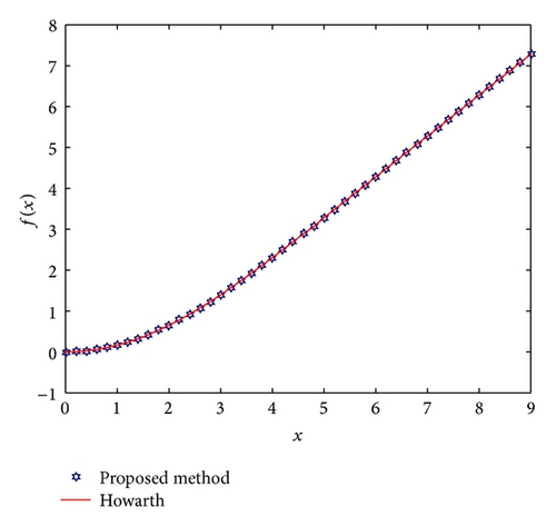
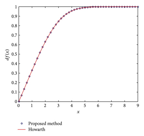
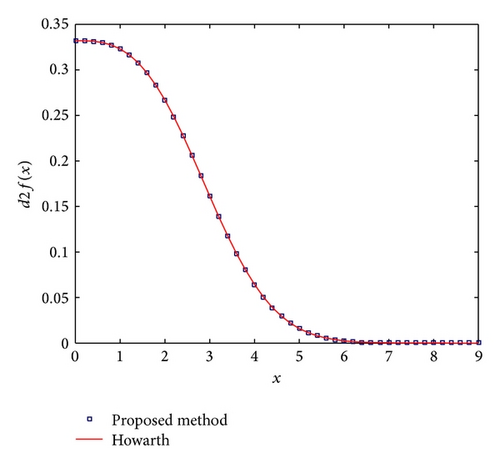
In this section, approximation values of f(x), f′(x), and f′′(x) based on proposed methods for some values of x are presented. These values for h = 0.2,0.1,0.01 have been calculated and these results are compared with the Howarth results. Tables 2, 3, and 4 are made to compare between the present results and results given by Howarth for approximation values of f(x), f′(x), and f′′(x), respectively. In Figures 1, 2, and 3, one can also see the comparison between our results and Howarth’s results.
| x | DTM [11] | LTNHPM [7] | Howarth (RK4) | Proposed method | ||
|---|---|---|---|---|---|---|
| h = 0.2 | h = 0.1 | h = 0.01 | ||||
| 0.0 | 0.00000 | 0.00000 | 0.00000 | 0.00000 | 0.00000 | 0.00000 |
| 0.2 | 0.00664 | 0.00664 | 0.00664 | 0.00664 | 0.00664 | 0.00664 |
| 0.4 | 0.02656 | 0.02656 | 0.02656 | 0.02656 | 0.02656 | 0.02656 |
| 0.6 | 0.05973 | 0.05973 | 0.05974 | 0.05973 | 0.05973 | 0.05973 |
| 0.8 | 0.10611 | 0.10611 | 0.10611 | 0.10609 | 0.10610 | 0.10611 |
| 1.0 | 0.16557 | 0.16557 | 0.16557 | 0.16554 | 0.16556 | 0.16557 |
| 1.2 | 0.23795 | 0.23795 | 0.23795 | 0.23790 | 0.23794 | 0.23795 |
| 1.4 | 0.32298 | 0.32298 | 0.32298 | 0.32290 | 0.32296 | 0.32298 |
| 1.6 | 0.42032 | 0.42032 | 0.42032 | 0.42021 | 0.42029 | 0.42032 |
| 1.8 | 0.52952 | 0.52952 | 0.52952 | 0.52936 | 0.52948 | 0.52952 |
| 2.0 | 0.65002 | 0.65002 | 0.65003 | 0.64982 | 0.64997 | 0.65002 |
| 2.2 | 0.78119 | 0.78119 | 0.78120 | 0.78093 | 0.78113 | 0.78119 |
| 2.4 | 0.92229 | 0.92228 | 0.92230 | 0.92197 | 0.92221 | 0.92229 |
| 2.6 | 1.07250 | 1.07250 | 1.07252 | 1.07212 | 1.07241 | 1.07250 |
| 2.8 | 1.23098 | 1.23098 | 1.23099 | 1.23054 | 1.23087 | 1.23098 |
| 3.0 | 1.39681 | 1.39681 | 1.39682 | 1.39631 | 1.39668 | 1.39681 |
| 3.2 | 1.56909 | 1.56909 | 1.56911 | 1.56854 | 1.56896 | 1.56909 |
| 3.4 | 1.74695 | 1.74695 | 1.74696 | 1.74635 | 1.74680 | 1.74695 |
| 3.6 | 1.92952 | 1.92952 | 1.92954 | 1.92889 | 1.92936 | 1.92952 |
| 3.8 | 2.11603 | 2.11602 | 2.11605 | 2.11536 | 2.11586 | 2.11603 |
| 4.0 | 2.30574 | 2.30575 | 2.30576 | 2.30506 | 2.30557 | 2.30574 |
| 4.2 | 2.49804 | 2.49805 | 2.49806 | 2.49733 | 2.49786 | 2.49804 |
| 4.4 | 2.69236 | 2.69242 | 2.69238 | 2.69164 | 2.69218 | 2.69236 |
| 4.6 | 2.88824 | 2.88859 | 2.88826 | 2.88751 | 2.88806 | 2.88824 |
| 4.8 | 3.08532 | 3.08718 | 3.08534 | 3.08458 | 3.08513 | 3.08532 |
| 5.0 | 3.28327 | 3.29272 | 3.28329 | 3.28252 | 3.28308 | 3.28327 |
| x | DTM [11] | LTNHPM [7] | Howarth (RK4) | Proposed method | ||
|---|---|---|---|---|---|---|
| h = 0.2 | h = 0.1 | h = 0.01 | ||||
| 0.0 | 0.00000 | 0.00000 | 0.00000 | 0.00000 | 0.00000 | 0.00000 |
| 0.2 | 0.06641 | 0.06641 | 0.06641 | 0.06640 | 0.06641 | 0.06641 |
| 0.4 | 0.13276 | 0.13276 | 0.13277 | 0.13275 | 0.13276 | 0.13276 |
| 0.6 | 0.19894 | 0.19894 | 0.19894 | 0.19890 | 0.19893 | 0.19894 |
| 0.8 | 0.26471 | 0.26471 | 0.26471 | 0.26465 | 0.26469 | 0.26471 |
| 1.0 | 0.32978 | 0.32978 | 0.32979 | 0.32969 | 0.32976 | 0.32978 |
| 1.2 | 0.39378 | 0.39378 | 0.39378 | 0.39365 | 0.39374 | 0.39378 |
| 1.4 | 0.45626 | 0.45626 | 0.45627 | 0.45610 | 0.45622 | 0.45626 |
| 1.6 | 0.51676 | 0.51676 | 0.51676 | 0.51656 | 0.51671 | 0.51676 |
| 1.8 | 0.57476 | 0.57476 | 0.57477 | 0.57452 | 0.57470 | 0.57476 |
| 2.0 | 0.62976 | 0.62977 | 0.62977 | 0.62950 | 0.62970 | 0.62976 |
| 2.2 | 0.68131 | 0.68131 | 0.68132 | 0.68102 | 0.68124 | 0.68131 |
| 2.4 | 0.72898 | 0.72898 | 0.72899 | 0.72868 | 0.72891 | 0.72898 |
| 2.6 | 0.77245 | 0.77245 | 0.77246 | 0.77215 | 0.77238 | 0.77245 |
| 2.8 | 0.81151 | 0.81151 | 0.81152 | 0.81122 | 0.81144 | 0.81151 |
| 3.0 | 0.84604 | 0.84604 | 0.84605 | 0.84577 | 0.84598 | 0.84604 |
| 3.2 | 0.87608 | 0.87608 | 0.87609 | 0.87584 | 0.87602 | 0.87608 |
| 3.4 | 0.90176 | 0.90176 | 0.90177 | 0.90155 | 0.90171 | 0.90176 |
| 3.6 | 0.92333 | 0.92333 | 0.92333 | 0.92315 | 0.92329 | 0.92333 |
| 3.8 | 0.94112 | 0.94112 | 0.94112 | 0.94098 | 0.94108 | 0.94112 |
| 4.0 | 0.95552 | 0.95553 | 0.95552 | 0.95541 | 0.95549 | 0.95552 |
| 4.2 | 0.96696 | 0.96704 | 0.96696 | 0.96688 | 0.96694 | 0.96696 |
| 4.4 | 0.97587 | 0.97639 | 0.97587 | 0.97581 | 0.97586 | 0.97587 |
| 4.6 | 0.98268 | 0.98564 | 0.98269 | 0.98264 | 0.98267 | 0.98268 |
| 4.8 | 0.98779 | 1.00322 | 0.98779 | 0.98775 | 0.98778 | 0.98779 |
| 5.0 | 0.99154 | 1.06671 | 0.99155 | 0.99151 | 0.99153 | 0.99154 |
| x | DTM [11] | LTNHPM [7] | Howarth (RK4) | Proposed method | ||
|---|---|---|---|---|---|---|
| h = 0.2 | h = 0.1 | h = 0.01 | ||||
| 0.0 | 0.33206 | 0.33206 | 0.33206 | 0.33206 | 0.33206 | 0.33206 |
| 0.2 | 0.33198 | 0.33198 | 0.33199 | 0.33195 | 0.33197 | 0.33198 |
| 0.4 | 0.33147 | 0.33147 | 0.33147 | 0.33140 | 0.33145 | 0.33147 |
| 0.6 | 0.33008 | 0.33008 | 0.33008 | 0.32997 | 0.33005 | 0.33008 |
| 0.8 | 0.32739 | 0.32739 | 0.32739 | 0.32725 | 0.32735 | 0.32739 |
| 1.0 | 0.32301 | 0.32301 | 0.32301 | 0.32284 | 0.32297 | 0.32301 |
| 1.2 | 0.31659 | 0.31659 | 0.31659 | 0.31641 | 0.31654 | 0.31659 |
| 1.4 | 0.30786 | 0.30786 | 0.30787 | 0.30767 | 0.30782 | 0.30786 |
| 1.6 | 0.29666 | 0.29666 | 0.29667 | 0.29648 | 0.29662 | 0.29666 |
| 1.8 | 0.28293 | 0.28293 | 0.28293 | 0.28276 | 0.28289 | 0.28293 |
| 2.0 | 0.26675 | 0.26675 | 0.26675 | 0.26662 | 0.26672 | 0.26675 |
| 2.2 | 0.24835 | 0.24835 | 0.24835 | 0.24826 | 0.24833 | 0.24835 |
| 2.4 | 0.22809 | 0.22809 | 0.22809 | 0.22805 | 0.22808 | 0.22809 |
| 2.6 | 0.20645 | 0.20645 | 0.20646 | 0.20647 | 0.20646 | 0.20645 |
| 2.8 | 0.18401 | 0.18401 | 0.18401 | 0.18408 | 0.18402 | 0.18401 |
| 3.0 | 0.16136 | 0.16136 | 0.16136 | 0.16148 | 0.16139 | 0.16136 |
| 3.2 | 0.13913 | 0.13913 | 0.13913 | 0.13928 | 0.13917 | 0.13913 |
| 3.4 | 0.11788 | 0.11788 | 0.11788 | 0.11805 | 0.11792 | 0.11788 |
| 3.6 | 0.09809 | 0.09809 | 0.09809 | 0.09827 | 0.09813 | 0.09809 |
| 3.8 | 0.08013 | 0.08014 | 0.08013 | 0.08030 | 0.08017 | 0.08013 |
| 4.0 | 0.06423 | 0.06436 | 0.06424 | 0.06438 | 0.06427 | 0.06423 |
| 4.2 | 0.05052 | 0.05131 | 0.05052 | 0.05064 | 0.05055 | 0.05052 |
| 4.4 | 0.03897 | 0.04360 | 0.03897 | 0.03906 | 0.03899 | 0.03897 |
| 4.6 | 0.02948 | 0.05446 | 0.02948 | 0.02954 | 0.02950 | 0.02948 |
| 4.8 | 0.02187 | 0.14672 | 0.02187 | 0.02190 | 0.02188 | 0.02187 |
| 5.0 | 0.01591 | 0.59821 | 0.01591 | 0.01591 | 0.01591 | 0.01591 |


4. Conclusion
In this survey, the quartic B-spline approximations are used to solve the Blasius equation. This method led to a system of nonlinear equations. The unknowns are obtained by minimizing the error norm. The computed results are compared with those of DTM, LTNHPM, and Howarth’s methods to demonstrate the validity and applicability of the technique. This method is simple in applicability and the results show that the solutions will become more accurate with reducing step size. The computations associated with the examples in this paper were performed using MATLAB R2015a.
Competing Interests
The authors of the paper do not have a direct financial relation that might lead to “competing interests” for any of the authors.


