This study concerns the development of a straightforward numerical technique associated with Classical Newton’s Method for providing a more accurate approximate solution of scalar nonlinear equations. The proposed procedure is based on some practical geometric rules and requires the knowledge of the local slope of the curve representing the considered nonlinear function. Therefore, this new technique uses, only as input data, the first-order derivative of the nonlinear equation in question. The relevance of this numerical procedure is tested, evaluated, and discussed through some examples.

1. Introduction

The resolution of nonlinear problems is an issue frequently encountered in several scientific fields such as mathematics, physics, or many engineering branches, for example, mechanics of solids [1–8]. In most cases, these problems are governed by nonlinear equations not having any analytical solution. In this regard, the introduction of iterative methods is therefore needed in order to provide a numerical approximate solution associated with any type of nonlinear equation [9–23]. Among these iterative algorithms, Classical Newton’s Method (CNM) [24, 25] is one of the most used mainly for the following reasons: (i) the simplicity for numerical implementation in any scientific computation software; (ii) the only knowledge of the first-order derivative of the considered function; (iii) the quadratic rate of convergence. In this paper, we propose a New Numerical Technique (NNT) based on geometric considerations which enable providing a more accurate approximate solution than that obtained by CNM. The present study is organized as follows: (i) in the first part, Section 2.1, we outline the scientific framework of this study, then, in second part, Section 2.2, we recall CNM including some convergence results, and, finally, in the third part, Section 2.3, we present NNT which uses only the first-order derivative of the considered nonlinear equation in order to enhance the predictive abilities of CNM; (ii) in Section 3, the numerical relevance of the proposed procedure is addressed, assessed, and discussed on some specific examples.

2. A New Numerical Technique (NNT) Combined with Classical Newton’s Method (CNM)

2.1. Problem Statement

We consider scalar-valued nonlinear equation

(with

) in the following form (see Figure 1):

()

where

denotes the class of infinitely differentiable functions in domain Ω, δ is the simple solution (so-called “simple true zero” or “simple root”) on interval

, that is, f(δ) = 0 with δ ∈ I.

Details are in the caption following the image — **Figure 1 (a)**
Open in figure viewer PowerPoint

Schematic diagram associated with the problem under consideration: monotonically increasing (a) and decreasing (b) nonlinear function f with a simple root δ on interval [a, b].

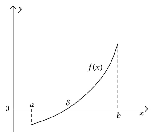
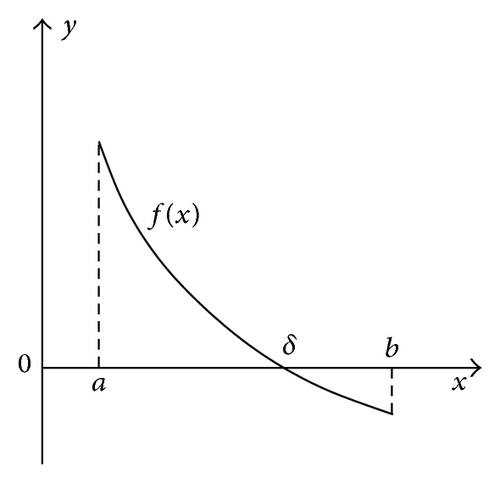
2.2. Classical Newton’s Method (CNM)

2.2.1. Iterative Algorithm

For using Classical Newton’s Method (CNM) [24, 25], we consider only the first-order term in Taylor series expansion associated with function f (i.e., the linearization of the considered function):

()

where f^′(p) denotes the first-order derivative of function f at point p.

The equation of tangent straight line T passing at point p = x^k ∈ I associated with function f is (∀x, y ∈ I; see Figure 2) as follows:

()

where †^k (resp., †^k+1) denotes kth (resp., (k + 1)th) iteration associated with variable † (with

Using (3), the linearization of (1) must check the following relation (∀x, y ∈ I and ∀x^k ∈ I):

()

Based on (4), (k + 1)th iterative point x^k+1 ∈ I provided by CNM is solution x = x^k+1 (∀x ∈ I) such as

()

2.2.2. Convergence Results

Considering Taylor series expansion of function f and truncation error (e^k) between kth iterative approximate solution (x^k) and true zero (δ), that is, e^k = x^k − δ (with ∀x^k ∈ I and δ ∈ I), we have

()

with

()

where f^[n](δ) denotes n-order derivative of function f at point δ (with

, n! is n-factorial,

represent the Higher-Order Terms which check:

, o(·) and

are Landau notations associated with the asymptotic behavior of function f, and ‖⋆‖ is the square norm or Euclidean-norm associated with the quantity ⋆ (here, Euclidean distance reduces to absolute value |⋆|, i.e., ‖⋆‖ ≡ |⋆|).

Since that f(δ) = 0, (6)-(7) can be written as follows (with ∀ x^k ∈ I):

()

The first-order derivative associated with function f at point x^k ∈ I (i.e., f^′(x^k)) checks:

()

Combining (5), (8)-(9), and x^k = δ + e^k leads to the following:

()

An iterative numerical scheme has θth order of convergence with associated convergence rate τ to number δ (i.e., “true zero”) if there exists θ ≥ 1 and τ ≥ 0 [25] such as

()

where |φ| is the absolute-value function of variable φ (such as | φ | = −φ when φ < 0, |φ| = 0 when φ = 0, and |φ| = φ when φ > 0) and “lim” is the limit operator. It is important to emphasize that (i) if θ = 1 and τ ∈ ]0,1[ then the convergence is linear (or “first-order” type, e.g., bisection or false position method); (ii) if θ = 1 and τ = 1 then the convergence is sublinear; (iii) if θ = 1 and τ = 0 (or θ > 1, ∀ τ ∈ ]0,1[) then the convergence is superlinear (e.g., secant method); (iv) if θ = 2 (with τ ∈ ]0,1[) then the convergence is quadratic (or “second-order” type, e.g., CNM); (v) if θ = 3 (with τ ∈ ]0,1[) then the convergence is cubic (or “third-order” type, e.g., TMNM; see Section 3.1). θth order of convergence means that the number of significant digits is θ-fold at each iteration k, for example, in the case of CNM (resp., TMNM), where θ = 2 (resp., θ = 3), the number of exact decimals doubles (resp., triples) at each iteration k.

Using (10)-(11), we can see that CNM has quadratic convergence (θ = 2) with a rate of convergence [24]:

()

2.3. New Numerical Technique (NNT)

2.3.1. Proposed Iterative Procedure

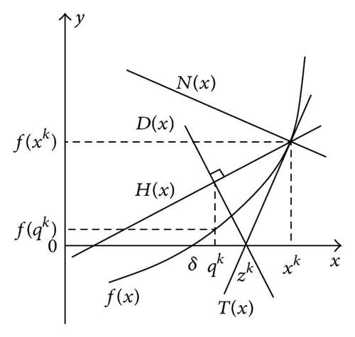
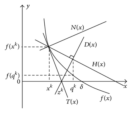
In this section, we propose a New Numerical Technique (NNT) for improving the accuracy associated with the approximate solution provided by CNM (see Section 2.2, which is used for finding the roots of scalar nonlinear equations. NNT is based on some practical geometric rules and requires only the determination of the local slope of the curve representing the considered nonlinear equation taking into account the first-order derivation (see [26–28]).

Here, we present the main steps associated with the development of NNT:

(i)
We consider normal straight line N associated with the curve representing nonlinear equation f at point x^k ∈ I (see [26, 27] and Figure 2):
()
(ii)
We introduce straight line H having direction vector which depends on the sum of direction vectors associated with normal and tangent straight lines passing by point (x^k, f(x^k)) (with ∀x^k ∈ I; see Figure 2), that is:
()
with
()
where w₁ = u₁ + v₁ and w₂ = u₂ + v₂ are the components of direction vector associated with straight line H in any orthonormal basis .
(iii)
Using CNM, we define kth iterative point z^k ∈ I (with ∀x ∈ I; see (5) and also Figure 2):
()
(iv)
We introduce also straight line D in the following form (with ∀x ∈ I; see Figure 2):
()
with
()
(v)
Combining (14)-(15) and (17)-(18), we adopt the solution x = q^k ∈ I of the equation H(x) = D(x) (with ∀x ∈ I; see Figure 2), that is:
()
According to (16) and (19), kth iterative point q^k ∈ I associated with NNT (see Figure 2) can be rewritten (with ∀x^k ∈ I):
()

The iterative numerical scheme associated with NNT is coupled with CNM and therefore (k + 1)th iterative solution x^k+1 ∈ I can be written as follows (with, ∀q^k, z^k ∈ I; see Figure 2):

()

with the different conditions associated with the iterative solution [A] (with ∀q^k, z^k, x^k ∈ I):

(i)
First condition [A1]: sgn⁡ (q^k) = sgn⁡ (x^k) and sgn⁡ (f(q^k)) = sgn⁡ (f(x^k)) and |f(q^k)| < |f(z^k)|.
(ii)
Second condition [A2]: |f(q^k)| < |f(z^k)|.

2.3.2. Convergence Analysis

Similar to that in Section 2.2.2, we analyze the convergence associated with NNT which is presented in Section 2.2.

Using (9) leads to the following:

()

In line with (22), we have the following:

()

On the other hand, we have the following:

()

Combining (8) and (24) leads to the following:

()

According to (19) and using (23) and (25), it holds that

()

In line with (11) and (26), we can see that the rate of convergence τ associated with NNT is

()

and the order of convergence is of linear-type (i.e., θ = 1) if 0 < τ_NNT ≤ 1 and quadratic-type (i.e., θ = 2) if τ_NNT = 0.

By taking (12) and (27), the rate of convergence τ_NNT-CNM of NNT combined with CNM is

()

It is important to emphasize that the associated convergence order is linear-type (θ = 1) if 0 < τ_NNT ≤ 1 with condition [A] (i.e., [A1] or [A2]) and quadratic-type (θ = 2) if τ_NNT = 0 with condition [A] (i.e., [A1] or [A2]) and elsewhere with τ_CNM ≠ 0.

3. Numerical Examples

3.1. Some Preliminary Remarks

In this section, we propose to test, evaluate, and analyze the iterative numerical procedure presented in Section 2.3 on some particular examples. This New Numerical Technique (NNT) is coupled with Classical Newton’s Method (CNM) in order to provide a more accurate approximate solution associated with scalar nonlinear equations. The numerical predictions obtained by combining both NNT and CNM are compared with those provided by Third-order Modified Newton’s Method (TMNM) [22, 26]. All numerical results presented here have been made with Matlab software (see [25, 29–32]).

For stopping the iterative process associated with each considered algorithm, we adopt three coupled types of Convergence Criterion (CC):

()

where K_max denotes the maximum number of iterations and ϵ_re (resp., ϵ_ae) is the tolerance parameter associated with the residue (resp., approximation) error criterion. Here, the considered values for each CC are K_max = 10, ϵ_re = 10⁻¹⁰, and ϵ_ae = 10⁻¹⁰.

The iterative numerical scheme associated with TMNM (see [22, 26]) is

()

where f^′′(x^k) denotes the second-order derivative of function f at point x^k. It should be noted that order of convergence θ is cubic (i.e., θ = 3) and rate of convergence τ is (see [22, 26])

()

3.2. Examples

We consider the following scalar nonlinear equations:

()

where exp⁡ (·), ln⁡ (·), and cos⁡ (·) represent exponential, natural logarithm, and cosinus functions.

The approximate numerical solution of roots associated with functions f₁, f₂, and f₃ are, respectively,

()

3.3. Results and Discussion

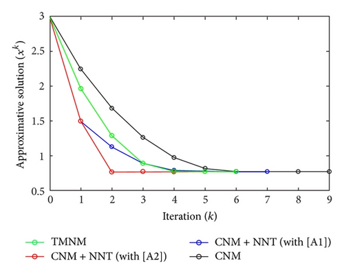
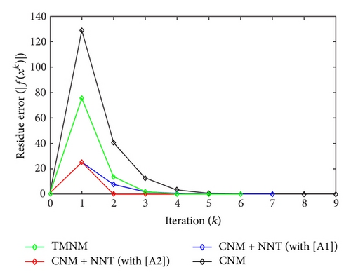
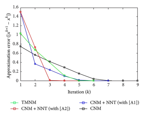
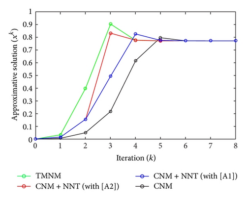
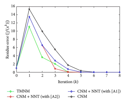
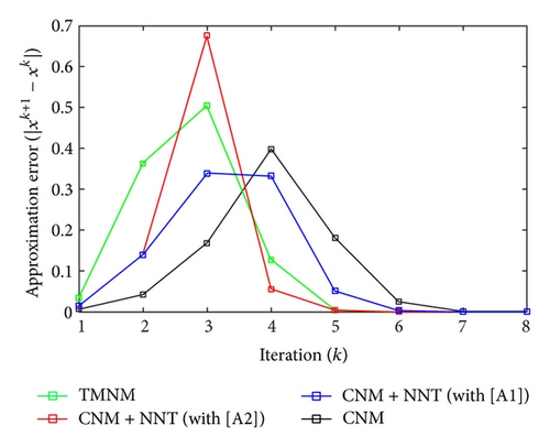
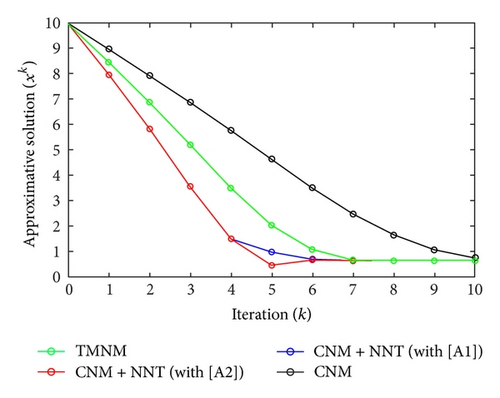
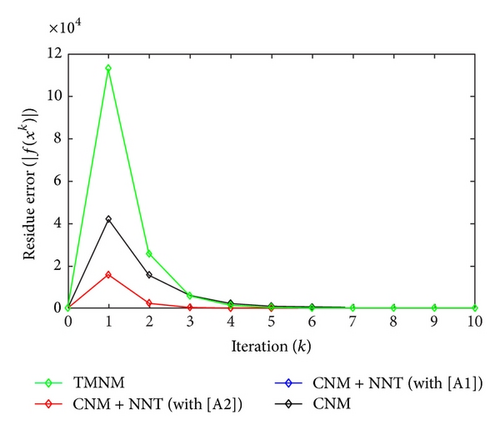
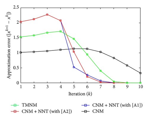
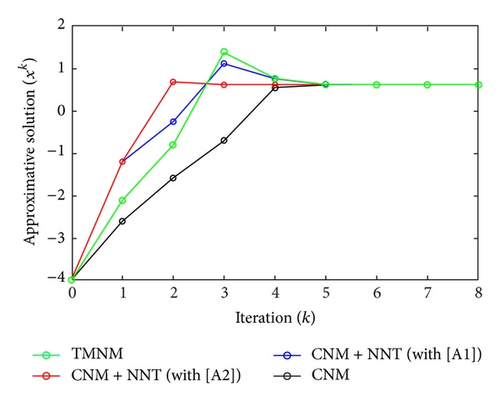
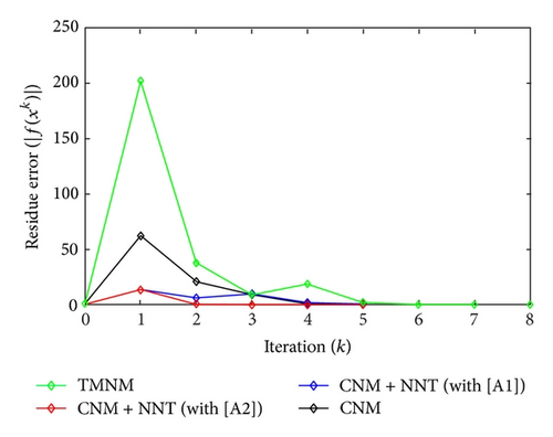
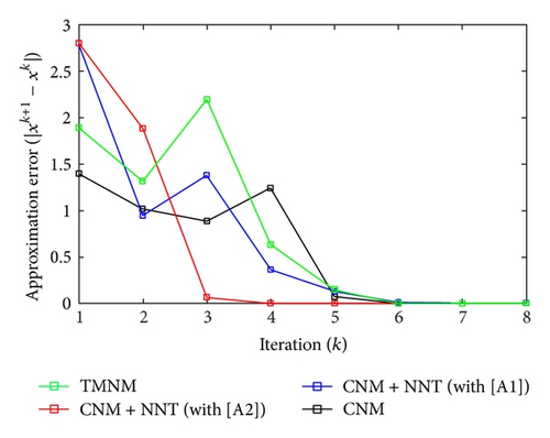
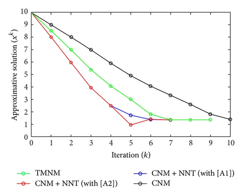
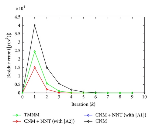
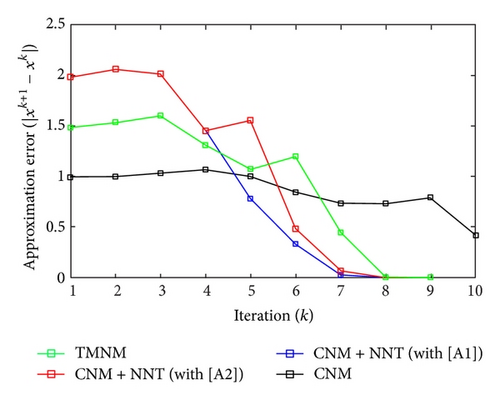
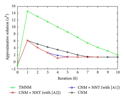
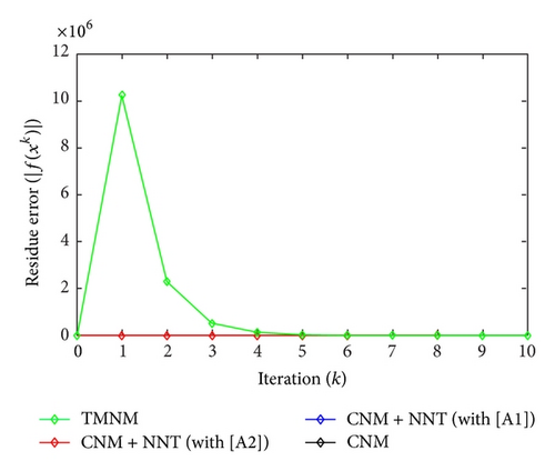
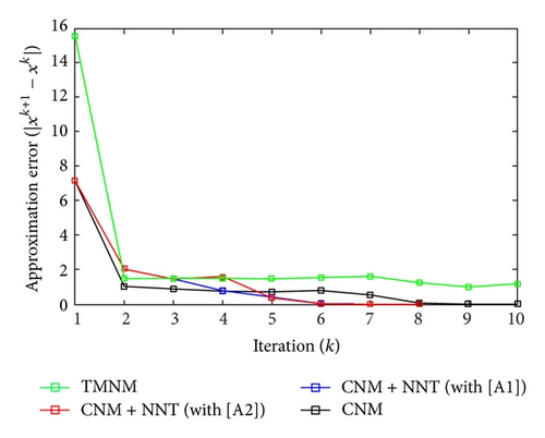
All the numerical results associated with scalar nonlinear functions f₁ to f₃ are presented in Tables 1–6 and also in Figures 3–20. For each scalar nonlinear function f_j (with j = 1,2, 3), we test two guest points x⁰ for starting iterative procedure: (i) in the case of function f₁, we adopt the first-guest point x⁰ = 3 (resp., second-guest point x⁰ = 10⁻³) and we show different approximate solutions x^k (with k = 1, …, 10) and also the evolution of both residue error |f(x^k+1)| and approximation error |x^k+1 − x^k| provided by Classical Newton’s Method (CNM; see Section 2.2), CNM coupled to the proposed New Numerical Technique (NNT) with both conditions [A1] and [A2] (CNM + NNT; see Section 2.3), and Third-order Modified Newton’s Method (TMNM; see Section 3.1) in Table 1 (resp., Table 2) and Figures 3–5 (resp., Figures 6–8); (ii) in the case of function f₂, we adopt first-guest point x⁰ = 10 (resp., second-guest point x⁰ = −4) and we show different approximate solutions x^k (with k = 1, …, 10) provided by CNM, CNM + NNT with both conditions [A1] and [A2], and TMNM in Table 3 (resp., Table 4) and Figures 9–11 (resp., Figures 12–14); (iii) in the case of function f₃, we adopt first-guest point x⁰ = 10 (resp., second-guest point x⁰ = −1) and we show different approximate solutions x^k (with k = 1, …, 10) provided by CNM, CNM + NNT with both conditions [A1] and [A2], and TMNM in Table 5 (resp., Table 6) and Figures 15–17 (resp., Figures 18–20). The obtained numerical results emphasize clearly that NNT combined with CNM is able to provide in the vast majority of cases a better approximate solution than that supplied only by CNM. In addition, on all results presented, condition [A2] seems to be more convenient than condition [A1]. For summary, NNT presents the main advantages of being a procedure: (i) “accurate” in terms of achieved approximate solution; (ii) “straightforward” to implement in computation software.

Table 1. Approximate solution x^k of scalar nonlinear equation f₁ (when guest point x⁰ = 3) obtained by Classical Newton’s Method (CNM) (cf. Section 2.2), Classical Newton’s Method coupled with New Numerical Technique (CNM + NNT) for conditions [A1] and [A2] (cf. Section 2.3), and Third-order Modified Newton’s Method (TMNM) (cf. Section 3.1). Notations: (∗∗) (resp., (∗)) denotes that approximate solution x^k is provided using (21a) (resp., (21b)) in Section 2.3.1.

Iteration (k)	CNM	CNM + NNT with condition [A1]	CNM + NNT with condition [A2]	TMNM
0	3.0000000000	3.0000000000	3.0000000000	3.0000000000
1	2.2471426305	1.4942904056 (∗∗)	1.4942904056 (∗∗)	1.9644439737
2	1.6823826593	1.1286469200 (∗)	0.7631581663 (∗∗)	1.2884809024
3	1.2337388302	0.8906377962 (∗)	0.7721173336 (∗)	0.8906149334
4	0.9723200229	0.7878458749 (∗)	0.7720250356 (∗)	0.7746164630
5	0.8146707520	0.7723183427 (∗)	0.7720250256 (∗)	0.7720250503
6	0.7741430851	0.7720251266 (∗)		0.7720250256
7	0.7720302909	0.7720250256 (∗)
8	0.7720250256
9	0.7720250256
10

Table 2. Approximate solution x^k of scalar nonlinear equation f₂ (when guest point x⁰ = 10⁻³) obtained by Classical Newton’s Method (CNM) (cf. Section 2.2), Classical Newton’s Method coupled with New Numerical Technique (CNM + NNT) for conditions [A1] and [A2] (cf. Section 2.3), and Third-order Modified Newton’s Method (TMNM) (cf. Section 3.1). Notations: (∗∗) (resp., (∗)) denotes that approximate solution x^k is provided using (21a) (resp., (21b)) in Section 2.3.1.

Iteration (k)	CNM	CNM + NNT with condition [A1]	CNM + NNT with condition [A2]	TMNM
0	0.0010000000	0.0010000000	0.0010000000	0.0010000000
1	0.0082410886	0.0154821756 (∗∗)	0.0154821756 (∗∗)	0.0344577770
2	0.0505339927	0.1548613133 (∗∗)	0.1548613133 (∗∗)	0.3980194000
3	0.2182202963	0.4938846484 (∗)	0.8311197179 (∗∗)	0.9031891893
4	0.6163033790	0.8261543800 (∗)	0.7760693275 (∗)	0.7755098327
5	0.7975366151	0.7754244611 (∗)	0.7720442199 (∗)	0.7720250858
6	0.7727863680	0.7720385875 (∗)	0.7720250260 (∗)	0.7720250256
7	0.7720257060	0.7720250258 (∗)	0.7720250256 (∗)
8	0.7720250256	0.7720250256 (∗)
9
10

Table 3. Approximate solution x^k of scalar nonlinear equation f₂ (when guest point x⁰ = 10) obtained by Classical Newton’s Method (CNM) (cf. Section 2.2), Classical Newton’s Method coupled with New Numerical Technique (CNM + NNT) for conditions [A1] and [A2] (cf. Section 2.3), and Third-order Modified Newton’s Method (TMNM) (cf. Section 3.1). Notations: (∗∗) (resp., (∗)) denotes that approximate solution x^k is provided using (21a) (resp., (21b)) in Section 2.3.1.

Iteration (k)	CNM	CNM + NNT with condition [A1]	CNM + NNT with condition [A2]	TMNM
0	10.000000000	10.000000000	10.000000000	10.000000000
1	8.9811766535	7.9623533071 (∗∗)	7.9623533071 (∗∗)	8.4655416573
2	7.9456740785	5.8372149905 (∗∗)	5.8372149905 (∗∗)	6.8799380466
3	6.8825672128	3.5600762341 (∗∗)	3.5600762341 (∗∗)	5.2048513181
4	5.7803883041	1.4821734803 (∗∗)	1.4821734803 (∗∗)	3.4865001565
5	4.6404493806	0.9609028311 (∗)	0.4402289741 (∗∗)	2.0197617679
6	3.5056070182	0.6928062817 (∗)	0.6483081663 (∗)	1.0685736902
7	2.4744259573	0.6233620739 (∗)	0.6199084714 (∗)	0.6632122684
8	1.6461067325	0.6192585092 (∗)	0.6192453069 (∗)	0.6193191836
9	1.0635449602	0.6192449541 (∗)	0.6192449540 (∗)	0.6192449540
10	0.7354406002	0.6192449510 (∗)		0.6192449540

Table 4. Approximate solution x^k of scalar nonlinear equation f₂ (when guest point x⁰ = −4) obtained by Classical Newton’s Method (CNM) (cf. Section 2.2), Classical Newton’s Method coupled with New Numerical Technique (CNM + NNT) for conditions [A1] and [A2] (cf. Section 2.3), and Third-order Modified Newton’s Method (TMNM) (cf. Section 3.1). Notations: (∗∗) (resp., (∗)) denotes that approximate solution x^k is provided using (21a) (resp., (21b)) in Section 2.3.1.

Iteration (k)	CNM	CNM + NNT with condition [A1]	CNM + NNT with condition [A2]	TMNM
0	−4.0000000000	−4.0000000000	−4.0000000000	−4.0000000000
1	−2.5987493208	−1.1976336149 (∗∗)	−1.1976336149 (∗∗)	−2.1088093909
2	−1.5803235380	−0.2513579056 (∗)	0.6858578709 (∗∗)	−0.7930763263
3	−0.6950023819	1.1303884977 (∗)	0.6226379112 (∗)	1.4022343921
4	0.5489290102	0.7665675348 (∗)	0.6192541648 (∗)	0.7698587570
5	0.6234126286	0.6349082108 (∗)	0.6192449540 (∗)	0.6217981372
6	0.6192588436	0.6194395336 (∗)	0.6192449540 (∗)	0.6192449694
7	0.6192449541	0.6192449843 (∗)		0.6192449540
8	0.6192449540	0.6192449540 (∗)		0.6192449540
9
10

Table 5. Approximate solution x^k of scalar nonlinear equation f₃ (when guest point x⁰ = 10) obtained by Classical Newton’s Method (CNM) (cf. Section 2.2), Classical Newton’s Method coupled with New Numerical Technique (CNM + NNT) for conditions [A1] and [A2] (cf. Section 2.3), and Third-order Modified Newton’s Method (TMNM) (cf. Section 3.1). Notations: (∗∗) (resp., (∗)) denotes that approximate solution x^k is provided using (21a) (resp., (21b)) in Section 2.3.1.

Iteration (k)	CNM	CNM + NNT with condition [A1]	CNM + NNT with condition [A2]	TMNM
0	10.000000000	10.000000000	10.000000000	10.000000000
1	9.0104267607	8.0208535216 (∗∗)	8.0208535216 (∗∗)	8.5171506533
2	8.0146859130	5.9615544966 (∗∗)	5.9615544966 (∗∗)	6.9859301990
3	6.9847503720	3.9493415483 (∗∗)	3.9493415483 (∗∗)	5.3851997390
4	5.9189110435	2.4996523082 (∗∗)	2.4996523082 (∗∗)	4.0778432768
5	4.9180876708	1.7226271036 (∗)	0.9467658294 (∗∗)	3.0067861343
6	4.0738875311	1.3881795157 (∗)	1.4273487664 (∗)	1.8098899052
7	3.3404588095	1.3598140013 (∗)	1.3607723321 (∗)	1.3648044141
8	2.6091363141	1.3595986336 (∗)	1.3595989925 (∗)	1.3595986468
9	1.8194405679	1.3595986211 (∗)	1.3595986211 (∗)	1.3595986211
10	1.4045600984

Table 6. Approximate solution x^k of scalar nonlinear equation f₃ (when guest point x⁰ = −1) obtained by Classical Newton’s Method (CNM) (cf. Section 2.2), Classical Newton’s Method coupled with New Numerical Technique (CNM + NNT) for conditions [A1] and [A2] (cf. Section 2.3), and Third-order Modified Newton’s Method (TMNM) (cf. Section 3.1). Notations: (∗∗) (resp., (∗)) denotes that approximate solution x^k is provided using (21a) (resp., (21b)) in Section 2.3.1.

Iteration (k)	CNM	CNM + NNT with condition [A1]	CNM + NNT with condition [A2]	TMNM
0	−1.0000000000	−1.0000000000	−1.0000000000	−1.0000000000
1	6.1409303723	6.1409303723 (∗)	6.1409303723 (∗)	14.5343055115
2	5.1148208484	4.0887116616 (∗∗)	4.0887116616 (∗∗)	13.0337347682
3	4.2379703013	2.6194618995 (∗∗)	2.6194618995 (∗∗)	11.5318478151
4	3.4892766889	1.8291595323 (∗)	1.0397597354 (∗∗)	10.0370297219
5	2.7676801225	1.4064394475 (∗)	1.3966765848 (∗)	8.5556896133
6	1.9776897481	1.3601688047 (∗)	1.3599586541 (∗)	7.0203746257
7	1.4417009128	1.3595987088 (∗)	1.3595986561 (∗)	5.3974911835
8	1.3613036994	1.3595986211 (∗)	1.3595986211 (∗)	4.1321703085
9	1.3595994046			3.1258556869
10	1.3595986211			1.9485648236

4. Concluding Comments

This study is devoted to a New Numerical Technique (NNT) to improve the accuracy of approximate solution provided by Classical Newton’s Method (CNM) and afford to have better numerical evaluation of the roots associated with the scalar nonlinear equations. As in CNM, this NNT requires only the determination of the first-order derivative of the nonlinear function under consideration. The predictive capabilities associated with NNT are shown on some examples.

Competing Interests

The author declares that they have no competing interests.

References

1 Nguyen Q. S., Stability and Nonlinear Solid Mechanics, 2000, John Wiley & Sons, New York, NY, USA.
Google Scholar
2 Doghri I., Mechanics of Deformable Solids: linear, Nonlinear, Analytical And Computational Aspects, 2000, Springer, Berlin, Germany, https://doi.org/10.1007/978-3-662-04168-0, MR1985282.
10.1007/978-3-662-04168-0
Web of Science® Google Scholar
3 Curnier A., Méthodes Numériques en Mécanique des Solides, 2000, Presses Polytechniques et Universitaires Romandes.
Google Scholar
4 Parnes R., Solid Mechanics in Engineering, 2001, Wiley, Hoboken, NJ, USA.
Google Scholar
5 Besson J., Cailletaud G., Chaboche J.-L., and Forest S., Non-Linear Mechanics of Materials, 2010, 167, Springer, Solid Mechanics and Its Applications.
10.1007/978-90-481-3356-7
Web of Science® Google Scholar
6 De Borst R., Crisfield M. A., Remmers J. J. C., and Verhoosel C. V., Non-Linear Finite Element Analysis of Solids and Structures. Computational Mechanics, 2012, Wiley-Blackwell, Hoboken, NJ, USA.
10.1002/9781118375938
Google Scholar
7 Bonnet M., Frangi A., and Rey C., The Finite Element Method in Solid Mechanics, 2014, McGraw-Hill Education.
Google Scholar
8 Kojić M. and Bathe K. J., Inelastic Analysis of Solids and Structures, 2005, Springer, Computational Fluid and Solid Mechanics.
Google Scholar
9 Abbasbandy S., Improving Newton-Raphson method for nonlinear equations by modified Adomian decomposition method, Applied Mathematics and Computation. (2003) 145, no. 2-3, 887–893, https://doi.org/10.1016/s0096-3003(03)00282-0, MR2009307, 2-s2.0-0042522428.
10.1016/S0096-3003(03)00282-0
Web of Science® Google Scholar
10 Noor M. A., New family of iterative methods for nonlinear equations, Applied Mathematics and Computation. (2007) 190, no. 1, 553–558, https://doi.org/10.1016/j.amc.2007.01.045, MR2338732, 2-s2.0-34249786251.
10.1016/j.amc.2007.01.045
Web of Science® Google Scholar
11 Noor K. I., Noor M. A., and Momani S., Modified Householder iterative method for nonlinear equations, Applied Mathematics and Computation. (2007) 190, no. 2, 1534–1539, https://doi.org/10.1016/j.amc.2007.02.036, MR2339744, 2-s2.0-34250658871.
10.1016/j.amc.2007.02.036
Web of Science® Google Scholar
12 Noor M. A., Some iterative methods free from second derivatives for nonlinear equations, Applied Mathematics and Computation. (2007) 192, no. 1, 101–106, https://doi.org/10.1016/j.amc.2007.02.138, MR2385573, 2-s2.0-34548440811.
10.1016/j.amc.2007.02.138
Web of Science® Google Scholar
13 Noor M. A., New classes of iterative methods for nonlinear equations, Applied Mathematics and Computation. (2007) 191, no. 1, 128–131, https://doi.org/10.1016/j.amc.2007.02.098, MR2385509, 2-s2.0-34547700484.
10.1016/j.amc.2007.02.098
Web of Science® Google Scholar
14 Chun C., A family of composite fourth-order iterative methods for solving nonlinear equations, Applied Mathematics and Computation. (2007) 187, no. 2, 951–956, https://doi.org/10.1016/j.amc.2006.09.009, MR2323101, 2-s2.0-34247261977.
10.1016/j.amc.2006.09.009
Web of Science® Google Scholar
15 Neta B. and Johnson A. N., High-order nonlinear solver for multiple roots, Computers & Mathematics with Applications. (2008) 55, no. 9, 2012–2017, https://doi.org/10.1016/j.camwa.2007.09.001, MR2401110, 2-s2.0-41049094793.
10.1016/j.camwa.2007.09.001
Web of Science® Google Scholar
16 Cordero A. and Torregrosa J. R., A class of multi-point iterative methods for nonlinear equations, Applied Mathematics and Computation. (2008) 197, no. 1, 337–344, https://doi.org/10.1016/j.amc.2007.07.047, MR2396315, ZBL1135.65322, 2-s2.0-38949167113.
10.1016/j.amc.2007.07.047
Web of Science® Google Scholar
17 Li T.-F., Li D.-S., Xu Z.-D., and Fang Y.-l., New iterative methods for non-linear equations, Applied Mathematics and Computation. (2008) 197, no. 2, 755–759, https://doi.org/10.1016/j.amc.2007.08.012, MR2400698, 2-s2.0-39449083002.
10.1016/j.amc.2007.08.012
Web of Science® Google Scholar
18 Chun C., A simply constructed third-order modifications of Newton′s method, Journal of Computational and Applied Mathematics. (2008) 219, no. 1, 81–89, https://doi.org/10.1016/j.cam.2007.07.004, MR2437697, 2-s2.0-45249110421.
10.1016/j.cam.2007.07.004
Web of Science® Google Scholar
19 Ham Y. M., Chun C., and Lee S.-G., Some higher-order modifications of Newton′s method for solving nonlinear equations, Journal of Computational and Applied Mathematics. (2008) 222, no. 2, 477–486, https://doi.org/10.1016/j.cam.2007.11.018, MR2474641, 2-s2.0-53449084497.
10.1016/j.cam.2007.11.018
Web of Science® Google Scholar
20 Fang L. and He G., Some modifications of Newton′s method with higher-order convergence for solving nonlinear equations, Journal of Computational and Applied Mathematics. (2009) 228, no. 1, 296–303, https://doi.org/10.1016/j.cam.2008.09.023, MR2514289, 2-s2.0-63349098348.
10.1016/j.cam.2008.09.023
Web of Science® Google Scholar
21 Chun C. and Neta B., Some modification of Newton′s method by the method of undetermined coefficients, Computers & Mathematics with Applications. (2008) 56, no. 10, 2528–2538, https://doi.org/10.1016/j.camwa.2008.05.005, 2-s2.0-53049083572.
10.1016/j.camwa.2008.05.005
Web of Science® Google Scholar
22 Antoni G., A new Newton-type method for solving both non-linear equations and systems, Asian Journal of Mathematics and Computer Research. (2015) 6, no. 3, 193–212.
Google Scholar
23 Antoni G., A new class of two-step iterative algorithms for finding roots of nonlinear equations, Asian Journal of Mathematics and Computer Research. (2015) 7, no. 3, 175–189.
Google Scholar
24 Kelley C. T., Solving Nonlinear Equations with Newton′s Method, 2003, 1, Society for Industrial and Applied Mathematics, Philadelphia, Pa, USA, Fundamental Algorithms for Numerical Calculations.
10.1137/1.9780898718898
Google Scholar
25 Quarteroni A., Sacco R., and Saleri F., Méthodes Numériques pour le Calcul Scientifique: Programmes en MATLAB, 2000, Springer, Berlin, Germany.
Google Scholar
26 Antoni G., A new iterative algorithm for approximating zeros of nonlinear scalar equations: geometry-based solving procedure, Asian Journal of Mathematics and Computer Research. (2015) 10, no. 2, 78–97.
Google Scholar
27 Antoni G., A new accurate and efficient iterative numerical method for solving the scalar and vector nonlinear equations: approach based on geometric considerations, International Journal of Engineering Mathematics. (2016) 2016, 18, 6390367, https://doi.org/10.1155/2016/6390367.
10.1155/2016/6390367
Google Scholar
28 Antoni G., A simple and efficient root-finding algorithm for dealing with scalar nonlinear equations: iterative procedure based on geometric considerations, Asian Journal of Mathematics and Computer Research. In press.
Google Scholar
29 Mathews J. H. and Fink K. K., Numerical Methods Using Matlab, 2004, Pearson.
Google Scholar
30 Yang W. Y., Cao W., Chung T. S., and Morris J., Applied Numerical Methods Using MATLAB, 2005, Wiley-Interscience, New York, NY, USA.
10.1002/0471705195
Web of Science® Google Scholar
31 Kiusalaas J., Numerical Methods in Engineering with MATLAB, 2009, Cambridge University Press, Cambridge, UK.
10.1017/CBO9780511812200
Google Scholar
32 Chapra S. C., Applied Numerical Methods with MATLAB for Engineers and Scientists, 2011, McGraw-Hill Higher Education.
Google Scholar

Citing Literature

All articles

An Efficient and Straightforward Numerical Technique Coupled to Classical Newton’s Method for Enhancing the Accuracy of Approximate Solutions Associated with Scalar Nonlinear Equations

Abstract

1. Introduction