Volume 2016, Issue 1 6268938

Research Article

Open Access

Climate Change Detection and Annual Extreme Temperature Analysis of the Amur River Basin

Bo Yan,

Corresponding Author

Bo Yan

[email protected]

orcid.org/0000-0001-7039-4402

College of Hydrology and Water Resources, Hohai University, Nanjing 20098, China hhu.edu.cn

State Key Laboratory of Hydrology-Water Resources and Hydraulic Engineering, Hohai University, Nanjing 20098, China hhu.edu.cn

Search for more papers by this author

Ziqiang Xia,

Ziqiang Xia

College of Hydrology and Water Resources, Hohai University, Nanjing 20098, China hhu.edu.cn

State Key Laboratory of Hydrology-Water Resources and Hydraulic Engineering, Hohai University, Nanjing 20098, China hhu.edu.cn

Search for more papers by this author

Feng Huang,

Feng Huang

College of Hydrology and Water Resources, Hohai University, Nanjing 20098, China hhu.edu.cn

State Key Laboratory of Hydrology-Water Resources and Hydraulic Engineering, Hohai University, Nanjing 20098, China hhu.edu.cn

Search for more papers by this author

Lidan Guo,

Lidan Guo

Business School, Hohai University, Nanjing 20098, China hhu.edu.cn

Search for more papers by this author

Xiao Zhang,

Xiao Zhang

College of Hydrology and Water Resources, Hohai University, Nanjing 20098, China hhu.edu.cn

State Key Laboratory of Hydrology-Water Resources and Hydraulic Engineering, Hohai University, Nanjing 20098, China hhu.edu.cn

Search for more papers by this author

Bo Yan,

Corresponding Author

Bo Yan

[email protected]

orcid.org/0000-0001-7039-4402

College of Hydrology and Water Resources, Hohai University, Nanjing 20098, China hhu.edu.cn

State Key Laboratory of Hydrology-Water Resources and Hydraulic Engineering, Hohai University, Nanjing 20098, China hhu.edu.cn

Search for more papers by this author

Ziqiang Xia,

Ziqiang Xia

College of Hydrology and Water Resources, Hohai University, Nanjing 20098, China hhu.edu.cn

State Key Laboratory of Hydrology-Water Resources and Hydraulic Engineering, Hohai University, Nanjing 20098, China hhu.edu.cn

Search for more papers by this author

Feng Huang,

Feng Huang

College of Hydrology and Water Resources, Hohai University, Nanjing 20098, China hhu.edu.cn

State Key Laboratory of Hydrology-Water Resources and Hydraulic Engineering, Hohai University, Nanjing 20098, China hhu.edu.cn

Search for more papers by this author

Lidan Guo,

Lidan Guo

Business School, Hohai University, Nanjing 20098, China hhu.edu.cn

Search for more papers by this author

Xiao Zhang,

Xiao Zhang

College of Hydrology and Water Resources, Hohai University, Nanjing 20098, China hhu.edu.cn

State Key Laboratory of Hydrology-Water Resources and Hydraulic Engineering, Hohai University, Nanjing 20098, China hhu.edu.cn

Search for more papers by this author

First published: 25 August 2016

https://doi.org/10.1155/2016/6268938

Citations: 9

Academic Editor: Jorge E. Gonzalez

Share a link

Email
Wechat
Bluesky

Abstract

This paper aims to detect climate change points and compare the extreme temperature changes with the average-value changes in the Amur River basin. The daily air temperatures of 44 stations in the Amur River basin were collected from April 1, 1954, to March 31, 2013. The change points for annual mean and extreme temperature in 44 individual stations and their average were detected by the Mann-Kendall test, respectively. The annual mean temperature changed during 1980s in terms of increased mean value and relative stable standard deviation. The annual maximum temperature from 31 stations mostly located in the central and northwest basin changed significantly, and their change points occurred mainly in 1990s. For the annual minimum temperature, 32 stations mainly located in the central basin had significant changes. The generalized extreme value distribution was fitted to the postchange point subseries of annual extreme temperature and the parameters were estimated by the maximum likelihood method. The 10/50/100-year return levels were estimated by the method of profile likelihood. For the areas in the central and Northwestern basin, the probability of occurrence of hot extremes increased, while the occurrence probability of cold extremes was decreased in the central basin under climate change.

1. Introduction

Climate change is an important global issue among international communities and academic researchers. A large number of studies have focused on analyzing variations of temperature in different places [1–3]. However, research on the effects of climate change on the international river is limited, and the potential impacts of climate change on water resources will lead to significant challenges to water resource protection and management of the nations sharing the same river basin, even conflicts and wars, especially in Middle East and Africa [4, 5]. For the Amur River basin, Yu et al. [6] observed an increasing trend in the annual mean temperature series by Mann-Kendall test method (M-K), and Novorotskii [7] confirmed that the rising trends of cold seasons (winter and spring) were greater than warm seasons (summer and autumn) by statistical analyses of monthly mean temperature in 16 observation stations. However, studies comparing extreme temperature changes with average-value changes are still very scarce. There is a general agreement that the increasing temperature has direct influence on the changes in temperature extremes and gives rise to aggravation in the frequency and intensity of extreme climate events such as rainstorm, drought, and flood [8, 9]. Many studies present that extreme climate events are more serious threats to keep human and natural systems in a fit condition than the average behaviors [10]. The interest focusing on extreme temperature and its variation has increased over the world [11]. In fact, as two aspects of the most studied extreme events, the occurrences of high and low temperature severely influence agriculture, human health, demand for energy, water resources, and the availability of drinkable water, among others [12]. Under climate change, or global warming, little changes in the mean value of temperature can lead to large variations in the scale and frequency of extreme events including extreme temperature [13]. Accordingly, it is indispensable to explore the variation characteristics of the extreme temperature compared with the mean value in the Amur River basin.

Climate change was first detected using the annual temperature data. For a river basin, the changes of both local and regional temperature should be taken into consideration. In that sense, the regional temperature was obtained by averaging the recorded value of 44 stations. Then the change points of annual mean and extreme temperature for individuals and region were detected by Mann-Kendall test, respectively, and finally, the descriptive statistics of subseries before and after change point were analyzed. Spatial distribution patterns were derived through interpolation using the Co-Kriging Considering Altitude (CKCA) method [14–16], which has a better interpolation accuracy than other common interpolation methods by cross-validation, as seen on subareas of the Amur River basin [14, 15].

The extreme value theory consists of two aspects of general definitions of extreme events. The first one is to group the data into blocks with equal length and pick up the maxima (minima) in every block such as monthly maximum 1-day rainfall and annual minimum wind speed, and the other one is to extract values over a proper threshold such as annual flood damage over 5 million dollars and daily rainfall amount above 20 mm [17–19]. Following the first definition, data is extracted to the annual maxima (minima) and forms the annual maximum (minimum) temperature series (AMTS). In this paper, it is appropriate to use the generalized extreme value distribution (GEV) to fit AMTS, and the chi-square goodness-of-fit test is employed to measure the rationality and accuracy of fitting. As a matter of fact, the GEV distribution has been widely used in climate extreme value analyses all over the world [20–25], including AMTS [2].

The objective of this study was to estimate temperature change and annual extreme temperature analysis from April 1, 1954, to March 31, 2013, in the Amur River basin. Understanding the climate change and the variation of the extreme temperature of this basin will be a foundation to solve problems related to water resources and environment preservation. The paper is organized as follows: a description of the study area and data are given in Section 2. The methods used in this study are given in Section 3. The annual mean temperature change is analyzed in Section 4.1. The GEV distribution is applied to the extreme temperature considering change point in Section 4.2. Some conclusions are given in Section 5.

2. Study Area and Data

2.1. Study Area

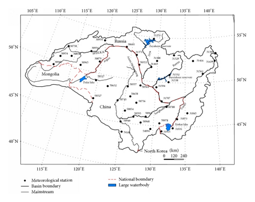
The Amur River (Figure 1), or Heilongjiang in Chinese, is both the eighth longest and tenth largest river in the world and also the most important international river in East Asia. The Amur River basin has an area of 1.86 million km² which covers the territories of Mongolia, Russia, China, and North Korea. In addition to its transboundary location, the Amur River basin can be characterized by contrasts between other geographical features: Russia and Asia; continental and monsoon climates; and Southern dense and northern sparse populations. The climate of Eastern Amur basin is humid monsoon climate, whose impact can reach the northernmost latitude, while the climate of areas in the west of this basin (upper reach of the Amur River) is sheltered from monsoon influence and arid. The arid western portion of this basin is smaller compared with the more humid Eastern portion [26].

Details are in the caption following the image — **Figure 1**
Open in figure viewer PowerPoint

Locations of the 44 meteorological stations in the Amur River basin.

2.2. Long-Term Observed Temperature Data

Identifying changes in climate extremes demands data quantity as well as data quality, compared with the study of changes in average behaviors. Even a relatively little amount of missing data may lead to the situation that an extreme event has not been recorded, especially when absolute extreme events are being studied [12].

The daily air temperature data from April 1, 1954, to March 31, 2013, were collected in this study, and the homogeneity of the data was controlled by the RHtestV.3 software package (http://etccdi.pacificclimate.org/software.shtml) which can be used to detect and adjust multiple shift points. Usually, these shift points exist in a data series that probably has first-order autoregressive errors. The penalized maximal F test (PMFT) inside this software is an improved method based on the common-trend two-phase regression model and used wildly to detect the multiple shift points in climate data. The detailed process of PMFT can be seen in literature [27, 28].

Spring lasts from April to May in the area of Amur River basin, summer lasts from June to August, autumn is from September to October, and winter starts from November and ends in March of the next year [29]. The climatic year is used to calculate AMTS instead of the calendar year, in order to avoid the situation that two continuous annual minima occurred in the same winter. April to March of the next year was considered as a climatic year; for example, 1 April 1954 to 31 March 1955 was considered as 1954. The annual maximum and minimum temperature were collected for every climatic year.

3. Methodology

The linear tendency estimate approach is used to analyze the changes in trend of annual mean and extreme temperature, combined with the least squares of the residuals, which is widely accepted to estimate the change rate of a time series. The Mann-Kendall rank statistical test (M-K) [30, 31] is employed to assess the statistical significance of a trend. As the M-K test is widely applied to test the trend [1] and detect abrupt changes [1, 32] in climate and hydrology time series, the temperature series for the individuals and area-averaged value of 44 stations are also detected to abrupt change points by M-K test in this study. For the annual temperature series x_i (1 ≤ i ≤ n), a sequence statistic S_k is calculated by

()

where x_i, x_j are data values of annual temperature; r_i is the rank statistic for the data pairs (x_i, x_j); S_k is the rank series; n is the length of the temperature series.

Under the null hypothesis of no trend, S_k is distributed as a normal distribution with the expected value of E(S_k) and the variance VAR(S_k) as follows:

()

Under the above assumption, the definition of the statistic index UF_k is calculated as

()

where UF_k is a standardized variable. Therefore, its sequential behavior fluctuates around zero level. A positive value indicates the upward trend of the temperature series, and vice versa.

Accordingly, the values of UB_k can be computed backward similarly as UF_k but starting from the end of the series; then UF_k and UB_k can be plotted to identify the change points.

The generalized extreme value (GEV) distribution is derived from the characterization of extreme behavior [2, 33]. Therefore it is appropriate to use for the annual extreme temperature series, as follows:

()

Defined on {z: 1 + ξ(z − μ)/σ > 0}, −∞ < μ < ∞ (location parameter), σ > 0 (scale parameter), and −∞ < ξ < ∞ (shape parameter), and the three extremal types are classified by the shape parameter: the Weibull distribution (ξ < 0), the Gumbel distribution (ξ = 0), and the Fréchet distribution (ξ > 0). The three parameters (

) are estimated by the maximum likelihood method (MLE).

Then the estimated values for quantiles of the GEV distribution are obtained in terms of the estimated parameters by MLE:

()

The chi-square goodness-of-fit test is used to evaluate the validity of the distribution with the MLE results, and its expression is as follows:

()

where O_i and E_i are the observed and expected frequencies for bin i, respectively. F is the cumulative distribution function of the tested distribution, and x₁, x₂ are the limits of the bin i. In this study, the result should be compared with the critical value

on account of three estimated parameters by MLE. If the result is smaller than the critical value, the GEV distribution fits well with the observed values and passes the test at a significant level α.

Estimating the return levels of annual extreme temperature events and how often the extreme quantiles occur with certain values are indispensable [33]. The interpretation of return level z(p) with return period T is as follows:

()

The profile likelihoods method (PLM) is used to improve the accuracy of the confidence intervals, and the confidence coefficient is set as 0.95. The profile likelihoods method aims to focus on the parameter of interest θ_i in a multiple parameter distribution, and θ_−i represents the remaining parameters. The logarithmic likelihood equation for θ_i can be expressed as

()

Based on the estimated parameters by MLE, the confidence interval for parameter of interest can be calculated by PLM, that is, the location parameter μ:

()

where c_1−α indicates the 1 − α quantile of chi-square distribution with 1 degree of freedom. According to the definition of GEV distribution, the relation between the quantiles and three parameters can be transformed as

()

When the quantiles z_p are attempted to be estimated by PLM, we just substitute (10) into (9) and take z_p as a constant value. Then the confidence interval for z_p is obtained by PLM.

When the annual minimum temperature is analyzed, the negative transformation of the data is fitted to the GEV distribution. For performing the extreme value analysis, an open source application R package extreme (http://www.assessment.ucar.edu/toolkit/) was used and it is well suitable for climate applications [2].

4. Results and Discussions

4.1. Annual Mean Temperature Abrupt Change Analysis

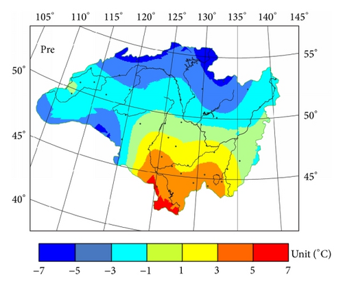
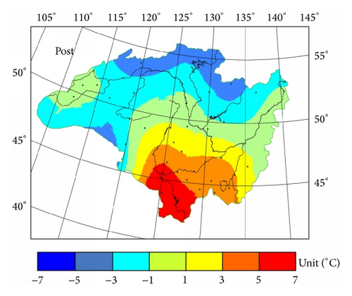
As seen in Table 1, the geographical location and altitude of 44 chosen stations were listed. The nonparametric M-K test (the confidence interval was set as 0.05) was used to detect climate change point for individual stations. The results of climate detection and descriptive statistics of the annual mean temperature, also shown in Table 1, confirmed that the change points of 44 stations were in the majority during 1980s, except for the stations of 30859, 31439, 31931, 50593, 50788, and 50978, whose change points were 1991, 1995, 1979, 1990, 1979, and 1979, respectively. Moreover, the frequency distribution of the change points for annual mean value was shown in Figure 2. 86.36% of stations with change points occurring in 1980s were detected based on the statistical result, and even 61.36% of stations had change points in the late 1980s. The statistical analyses of the pre- and postchange point subseries showed that the temperature increased significantly, and change patterns in individual stations were similar: the mean values increased and the standard deviations were relatively stable, and the increased magnitudes of the mean values ranged from 0.59 to 1.94°C. The spatial changes of the mean values for the pre- and postchange point subseries were shown in Figure 3, and CKCA was used to calculate spatial interpolation. The warming phenomenon occurred in the whole basin, and the high-value area became larger, while the low-value area was shrunken. As a whole, the annual mean temperature presented an obvious increase after change point in the Amur River basin.

Table 1. Climate change detection and descriptive statistics of the annual mean temperature series.

Meteorological station	Latitude (°N)	Longitude (°E)	Altitude (m)	Change point	Prechange		Postchange
Meteorological station	Latitude (°N)	Longitude (°E)	Altitude (m)	Change point	Mean value (°C)	Standard deviation (°C)	Mean value (°C)	Standard deviation (°C)
30673	53.75	119.73	624.00	1981	−5.28	0.79	−4.52	1.19
30758	52.08	113.48	671.00	1988	−2.67	0.08	−1.13	0.76
30777	52.23	117.70	528.00	1986	−3.24	0.89	−2.26	0.86
30859	51.10	114.52	680.00	1991	−1.53	0.77	−0.80	0.86
30879	51.32	119.62	621.00	1981	−3.05	0.94	−2.14	0.78
30965	50.40	116.52	675.00	1982	−2.55	0.97	−1.61	0.89
30954	50.70	112.67	807.00	1982	−0.87	0.74	0.11	0.82
30949	49.57	111.97	907.00	1982	−1.17	0.71	−0.47	0.81
50527	49.22	119.75	610.20	1982	−1.90	0.95	−0.38	1.03
30695	53.47	123.90	266.00	1981	−3.65	0.77	−2.70	0.72
31253	54.72	128.87	365.00	1986	−4.92	0.79	−3.63	0.87
31371	52.78	126.00	210.00	1985	−2.79	0.77	−1.54	0.76
31388	52.35	129.92	207.00	1983	−3.57	0.89	−2.47	0.86
31443	51.63	128.82	161.00	1985	−2.63	0.94	−1.36	0.90
50353	51.72	126.65	177.40	1984	−1.82	0.89	−0.20	0.87
31329	53.08	132.98	540.00	1988	−5.55	0.64	−4.32	0.66
31416	52.42	136.50	73.00	1989	−2.76	0.82	−1.57	0.61
31532	50.87	132.25	271.00	1986	−4.17	0.77	−2.82	0.85
31538	50.07	132.13	343.00	1985	−2.25	0.69	−1.11	0.72
31594	49.42	130.08	133.00	1988	−0.72	0.79	0.39	0.67
31707	47.73	130.97	72.00	1985	1.86	0.71	2.70	0.68
50564	49.43	127.35	234.50	1988	−1.33	0.80	0.61	0.65
31369	53.15	140.70	67.00	1989	−2.12	0.67	−1.52	0.60
31439	52.38	140.47	33.00	1995	−1.65	0.77	−0.75	0.48
31562	50.93	138.18	20.00	1989	−1.15	0.74	−0.45	0.43
31845	46.53	135.32	128.00	1988	0.52	0.56	1.40	0.54
31873	45.87	133.73	97.00	1985	2.46	0.70	3.21	1.16
31915	44.40	131.38	217.00	1981	4.00	0.66	4.59	0.64
31931	44.80	133.08	99.00	1979	3.20	0.74	3.86	0.68
50978	45.30	130.93	280.80	1979	3.63	0.69	4.50	0.70
50557	49.17	125.23	242.20	1985	−0.21	0.95	0.99	0.87
50593	45.75	126.77	142.30	1990	3.79	0.77	5.21	0.82
50632	48.77	121.92	739.70	1985	−0.88	0.72	0.00	0.72
50658	48.05	125.88	234.60	1986	1.29	0.84	2.42	0.81
50727	47.17	119.93	997.20	1989	−3.09	0.8	−2.04	0.63
50745	47.38	123.92	147.10	1986	3.37	0.81	4.51	0.82
50756	47.43	126.97	239.20	1987	1.49	0.80	2.68	0.76
50788	47.23	131.98	66.40	1979	2.55	0.76	3.37	0.73
50854	46.38	125.32	149.30	1988	3.31	0.79	4.44	0.75
50949	45.08	124.87	136.20	1981	4.60	0.79	5.80	0.85
50963	45.97	128.73	108.60	1989	2.36	0.74	3.17	0.68
50968	45.22	127.97	189.70	1988	2.41	0.72	3.72	0.72
54094	44.57	129.60	241.40	1986	3.66	0.78	4.90	0.70
54161	43.90	125.22	236.80	1987	5.03	0.77	6.34	0.80

The area-averaged annual mean temperature series was obtained by averaging the 44 stations. Figure 4 presented multiple trend analyses of slope estimator for periods with different start and end years. For the rationality and availability of statistical method, the length of these periods was limited to be more than 28 years. The results indicated strong significant positive trends in temperature with a rate of 0.03–0.55°C/decade. In particular, the strongest trend (0.55°C/decade) occurred in the period from 1968 to 1998, while the weakest trend (0.03°C/decade) occurred in the period from 1957 to 1987. It could be inferred that there might be a big step change for annual mean temperature in late 1980s. Furthermore, the bottom of the black contours in Figure 4 was around 1990 for the y-axis, which means that the increased trend turned significant (0.05 significance level) when the evaluation term was long enough (more than 30 years) and with an end year around 1990. It could also determine the conjecture that a big step change occurred in late 1980s, and the result was consistent with the individual stations’ statistical analyses above.

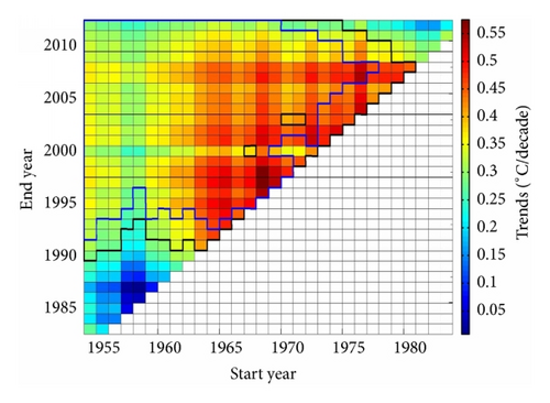
Figure 5 presented the changes of area-averaged annual mean temperature in the Amur River basin. The multiyear mean temperature was −0.09°C and the linear trend of annual mean temperature (0.30°C/decade) was positive. The result of M-K test showed that the significance of the trend change passed 0.01 confidence level. However, the high standard deviation (0.83°C) corresponded to the great interannual variation. One significant abrupt change which occurred in 1986 was detected in area-averaged annual mean temperature series and separated this series to two subseries. The multiyear mean value of the two subseries was −0.39 and 0.66°C, respectively.

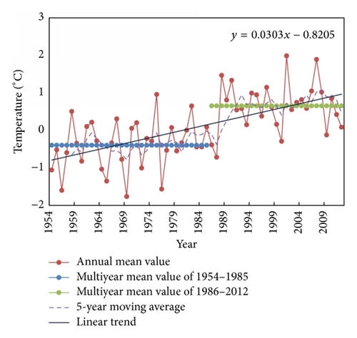
At the temporal scale, the climate of the Amur River basin has become significantly warmer in the past 59 years (Figure 5), similarly to Northeast Asia [8]. The significance of increasing trend for the area-averaged annual mean temperature was tested by M-K at 0.01 confidence level. This is consistent with the increasing trend in temperature detected by several other authors. Yu et al. [6] found a significant increase in annual mean temperature from 1950 to 2010, and Novorotskii [7] claimed that the tendency in temperature change in Amur River basin is generally synchronous to the global one, and the annual mean temperature increased by 1.3°C during the 20th century, based on the long-term observed data from 1891 to 2004. Panin et al. [34] demonstrated a similar conclusion at a bigger scale of the middle and high latitudes of the Northern Hemisphere, and Pan et al. [35] found that the temperature rose significantly since the 1980s in Heilongjiang province, which is in the Chinese part of the Amur River basin.

For the regional scale, the abrupt change of the annual mean temperature occurred during 1980s, combining the results of change detection for 44 individual stations series and their average. Overall, the annual mean temperature showed an increasing trend since 1980s. Consistent with our finding on the annual mean temperature, Pan and Zhang [36] detected the change point which occurred in 1990 in Heilongjiang province by moving t-test, and Sun et al. [37] employed the Yamamoto check method to detect the change point that occurred during 1987–1989 in Northeast China.

4.2. Extreme Temperature Analysis

4.2.1. Annual Maximum Temperature Abrupt Change Detection

The annual maximum temperature series was segmented into two subseries in agreement with climate change. The descriptive statistics of the maximum temperature subseries were listed in Table 2, and the frequency distribution of the change points was shown in Figure 6. There was no change point to be detected by M-K test in 13 stations, while 31 stations had change points, and their annual maximum temperature series were segmented. For the 13 stations without change point, it could be concluded that the annual maximum temperature of them changed slightly, and the segmentation of their series was canceled. For the subseries of annual maximum temperature in the 31 stations with change point, the mean value was increased, and 26 of 31 stations had the change points that occurred in 1990s. Considering the spatial distribution, the stations without change point in the annual maximum temperature are located mainly in the Eastern and Southern area of the Amur River.

Table 2. Climate change detection and descriptive statistics of the annual maximum temperature series.

Meteorological station	Change point	Prechange		Postchange
Meteorological station	Change point	Mean value (°C)	Standard deviation (°C)	Mean value (°C)	Standard deviation (°C)
30673	1998	21.18	1.47	22.50	1.20
30758	1994	23.19	1.71	25.26	1.80
30777	1997	23.69	1.66	25.28	1.70
30859	1998	23.00	1.73	24.83	1.88
30879	2000	23.10	1.63	24.51	2.03
30965	1997	25.08	1.89	27.11	2.29
30954	1997	22.99	1.49	25.67	2.04
30949	1997	21.85	1.39	24.24	2.11
50527	1988	24.89	1.69	26.46	1.80
30695	1998	23.80	1.62	25.07	1.34
31253	1998	23.04	1.31	24.43	1.46
31371	2000	24.58	1.54	26.27	1.69
31388	1996	23.92	1.29	25.01	1.15
31443	1998	24.49	1.23	25.96	1.53
50353	1993	25.53	1.50	27.53	1.95
31329	1998	21.43	1.02	23.09	1.19
31416	1997	24.84	1.50	25.68	1.88
31532	1994	23.17	1.10	24.95	1.38
31538	1997	23.49	1.30	24.92	1.64
31594	1997	25.48	1.10	26.85	1.08
31707	1994	25.66	1.26	26.51	1.34
50564	1994	24.43	1.16	26.46	1.63
31369	None			22.05	1.62
31439	None			22.93	1.52
31562	None			24.72	1.45
31845	None			25.08	1.32
31873	None			25.70	1.25
31915	None			25.85	1.42
31931	None			26.13	1.48
50978	None			27.03	1.41
50557	1988	25.61	1.45	27.35	1.68
50593	None			27.75	1.27
50632	1992	22.60	1.41	23.64	1.62
50658	1997	26.28	1.13	27.82	1.49
50727	1997	22.82	1.35	24.86	1.71
50745	1996	28.00	1.27	29.58	1.66
50756	1999	26.03	1.29	27.40	1.38
50788	1974	26.47	1.19	27.54	1.53
50854	None			28.02	1.38
50949	1997	27.77	1.08	28.54	1.40
50963	None			26.57	1.15
50968	1995	25.86	1.03	26.77	1.17
54094	None			27.14	1.21
54161	None			27.38	1.21

The “None” indicates no change point was detected by M-K test at 0.05 confidence level, and the descriptive statistics of the whole annual maximum temperature series are filled in the blank of the postchange subseries.

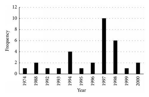
Figure 7 shows the changes of area-averaged annual maximum temperature in the Amur River basin. The multiyear mean temperature was 25.11°C and the linear trend (0.30°C/decade) was positive. The result of M-K test showed that the significance of change passed 0.01 confidence level. One significant abrupt change which occurred in 1995 was detected in area-averaged annual maximum temperature series and separated the series to two subseries. The multiyear mean values of the two subseries were 24.73 and 25.55°C, respectively.

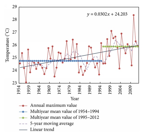
For the regional scale, the abrupt change of the annual maximum temperature in the basin occurred during 1990s, combining the results of change detection for 44 individual stations and their averaged value. For the local scale, the changes of the annual maximum temperature for the stations in east and south area of the Amur River basin were negligible.

4.2.2. Annual Maximum Temperature Return Levels Estimations

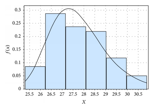
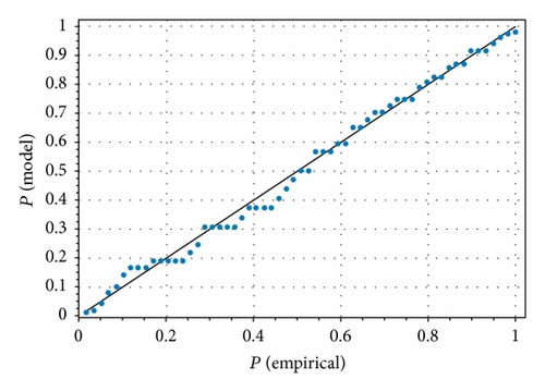
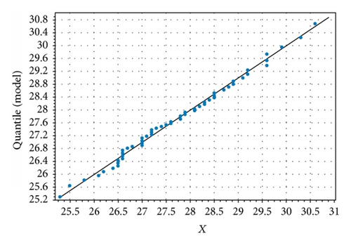
The GEV distribution was fitted to the annual maximum temperature series. The chi-square goodness-of-fit test results support the rationality of the GEV distribution for annual maximum temperature. 10/50/100-year return levels for annual maximum temperature were estimated by the profile likelihood method. For the stations with change point, the two subseries were fitted by the GEV distribution, respectively. For the stations without change point, the entire series of the annual maximum temperature was fitted. We took station 50593 as an example to introduce the process of chi-square goodness-of-fit test. The parameter estimates (, , ) for 50593 and their standard errors were listed in Table 3, and they were calculated by MLE. Particularly, the value of ξ corresponded to the Weibull distribution. The diagnosis graphs for fitting the annual maximum temperature in 50593 to GEV distribution were shown in Figure 8, including probability density function, P-P plot, and Q-Q plot. Both the P-P and Q-Q plots that deviated a little from the straight line suggested that the model fitted well with the observed values. As seen in Figure 8(a), frequency statistics were divided into 6 bins, and χ² was 1.21 following (7), which is smaller than , indicating that the GEV distribution was appropriate for fitting the annual maximum temperature in 50593 at 0.05 significance level.

Table 3. Parameter estimates for the GEV distribution by MLE.

Station	Location μ (°C)		Scale σ (°C)		Shape ξ
Station	Estimate	Standard error	Estimate	Standard error	Estimate	Standard error
50593	27.22	0.16	1.12	0.12	−0.13	0.10

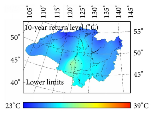
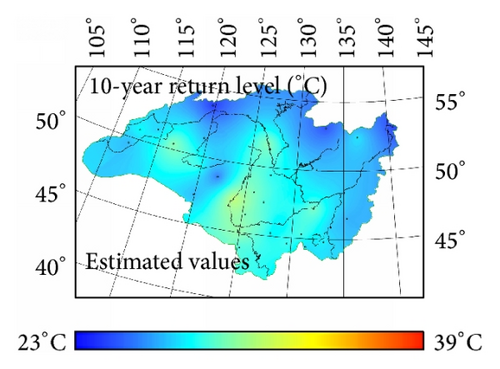
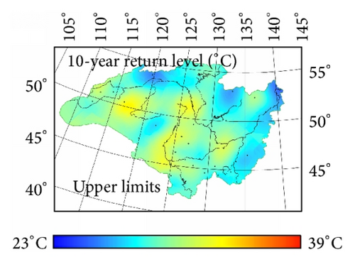
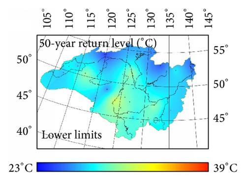
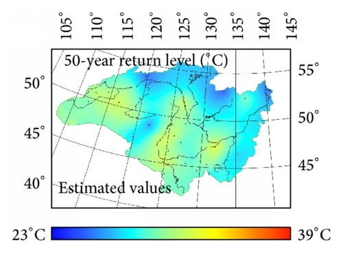
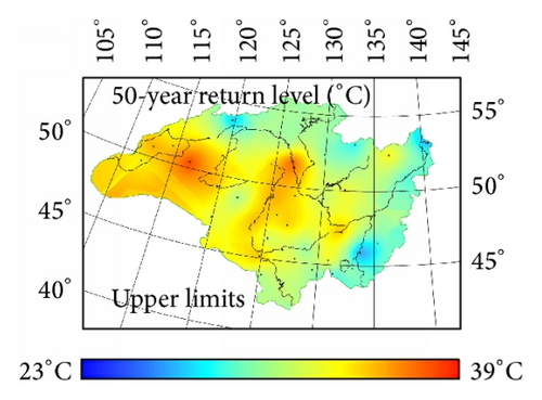
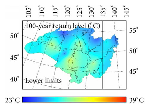
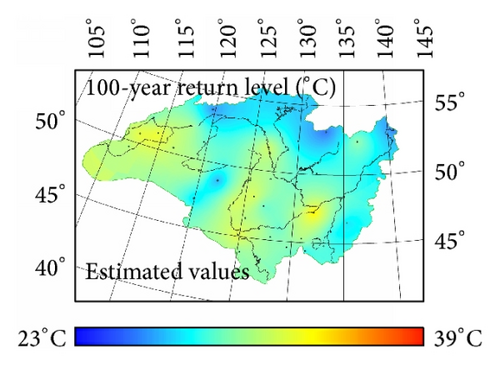
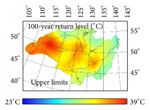
10/50/100-year return levels for annual maximum temperature were estimated by PLM. For the stations with change point, the postchange point subseries were fitted by the GEV distribution, while the entire series was fitted in stations without change points. Figure 9 showed the spatial distribution of 10/50/100-year return levels for the postchange point subseries of annual maximum temperature. Overall, the probability of occurrence of hot extremes significantly increased for Northwestern regions of the basin, while for partly east and south regions, moderated by the influence of the Seas of Okhotsk and Japan, the change point for the annual maximum temperature series was not detected, and the probability of hot extreme events increased inconspicuously.

4.2.3. Annual Minimum Temperature Abrupt Change Detection

The annual minimum temperature series was segmented into two subseries in agreement with detected change points. The descriptive statistics of the minimum temperature subseries were listed in Table 4, and the frequency distribution of the change points for annual minimum temperature was displayed in Figure 10. There was no change point detected by M-K test in 12 stations, while 32 stations had change points, and their annual minimum temperature series had been segmented. The change points in annual minimum temperature generally occurred earlier at almost all stations, compared with those in annual maximum values. For the subseries of annual minimum temperature, the mean value of stations increased. Taking into account the spatial distribution, the stations without change point in the annual minimum temperature were mainly in the Eastern and Northwestern basin.

Table 4. Climate change detection and descriptive statistics of the annual minimum temperature series.

Meteorological station	Change point	Prechange		Postchange
Meteorological station	Change point	Mean value ( ^°C)	Standard deviation ( ^°C)	Mean value ( ^°C)	Standard deviation ( ^°C)
30673	1975	−39.07	3.04	−37.53	3.02
30758	None			−35.79	2.57
30777	1966	−39.51	3.08	−37.61	3.02
30859	None			−32.71	3.05
30879	None			−35.38	2.88
30965	None			−35.67	3.35
30954	None			−30.45	3.05
30949	None			−30.24	3.02
50527	1972	−35.66	2.21	−33.33	2.99
30695	1982	−37.78	2.79	−36.93	2.66
31253	1988	−41.12	2.23	−38.19	3.01
31371	1975	−39.54	2.36	−37.6	3.53
31388	1983	−40.42	2.42	−38.37	2.42
31443	1981	−39.29	3.10	−37.01	2.67
50353	1982	−37.65	2.88	−34.22	2.92
31329	1981	−41.18	2.35	−39.72	2.27
31416	1983	−38.72	2.71	−36.52	2.6
31532	1983	−41.38	2.17	−39.11	2.16
31538	1981	−35.2	2.39	−33.79	2.01
31594	1988	−35.49	2.23	−33.88	2.65
31707	None			−27.15	2.61
50564	1988	−34.18	2.52	−31.45	2.75
31369	None			−32.02	2.97
31439	1999	−34.21	2.96	−31.66	1.69
31562	None			−35.26	2.39
31845	None			−31.75	2.09
31873	1990	−27.48	1.97	−25.79	2.26
31915	None			−22.27	2.22
31931	None			−27.39	2.73
50978	1989	−24.26	2.09	−22.73	2.41
50557	1971	−34.41	2.57	−32.3	3.21
50593	1991	−27.16	3.65	−24.08	2.96
50632	1982	−29.47	2.20	−28.15	2.39
50658	1971	−30.58	2.10	−28.61	2.78
50727	1979	−36.19	2.48	−34.4	2.43
50745	1988	−26.37	2.52	−24.79	3.39
50756	1990	−30.23	2.39	−28.05	2.65
50788	1988	−26.97	2.07	−26.05	2.69
50854	1987	−27.54	2.53	−25.06	3.00
50949	1980	−25.17	2.36	−23.31	3.30
50963	1988	−28.57	2.17	−27.34	2.97
50968	1994	−28.72	2.35	−26.33	2.92
54094	1980	−25.92	2.45	−23.48	2.59
54161	1982	−24.84	2.38	−23.15	2.82

The “None” indicates no change point was detected by M-K test at 0.05 confidence level, and the descriptive statistics of the entire annual minimum temperature series are filled in the blank of the postchange subseries.

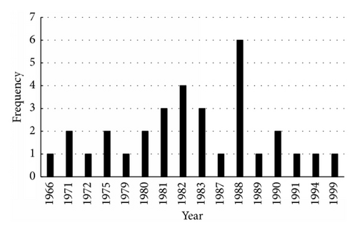
Figure 11 showed the changes of area-averaged annual minimum temperature in the Amur River basin. The multiyear mean temperature was −32°C and the linear trend of annual minimum temperature (0.40°C/decade) was positive. The result of the Mann-Kendall test showed that the change significance is lower than the 0.01 confidence level. One significant abrupt change which occurred in 1981 was detected in the annual minimum temperature series and separated the series into two subseries. The multiyear mean values of the two subseries were −32.85 and −31.32°C, respectively.

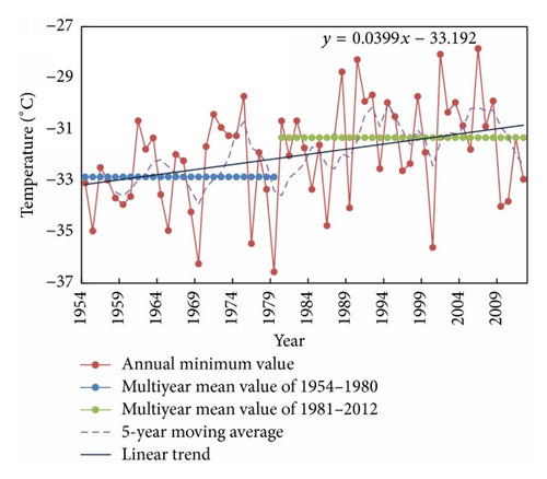
For the regional scale, the change point of the area-averaged series was not representative, even in the middle basin where most stations with change points were concentrated. The occurrence of change points for annual minimum temperature in 32 stations was decentralized, with local differences.

4.2.4. Annual Minimum Temperature Return Levels Estimations

The GEV distribution was fitted to the annual minimum temperature series using negative transformed data. The chi-square goodness-of-fit test results support the rationality of the GEV distribution for annual minimum temperature. 10/50/100-year return levels for annual minimum temperature were estimated by PLM. For the stations with change point, the postchange point subseries were fitted by the GEV distribution, while the entire series was fitted in stations without change points. Figure 12 displayed the spatial distribution of 10/50/100-year return levels for the postchange point subseries of annual minimum temperature. Overall, for the central regions of the basin, the probability of occurrence of cold extremes increased, while for the regions in the Eastern and Northwestern basin, moderated by the influences of the maritime climate and Siberian High in winter, respectively, the annual minimum temperature changed slightly.

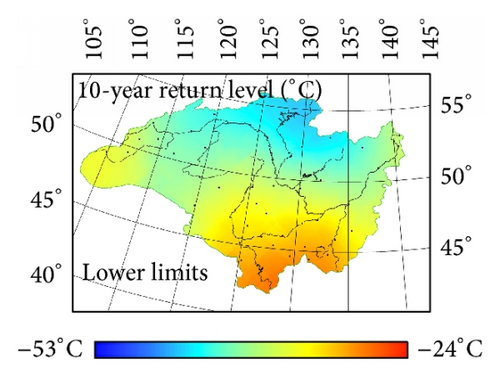
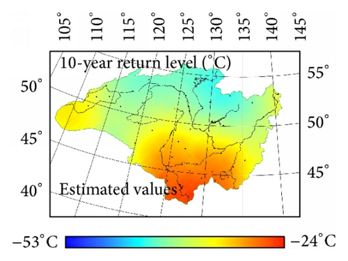
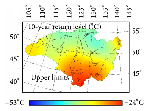
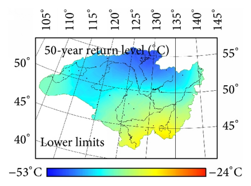
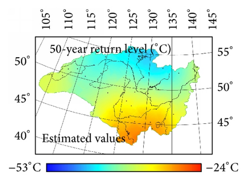
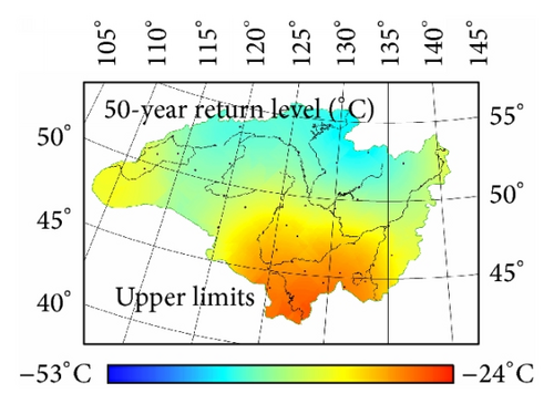
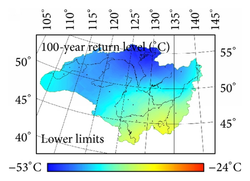
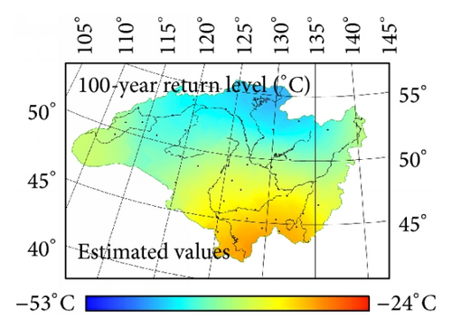
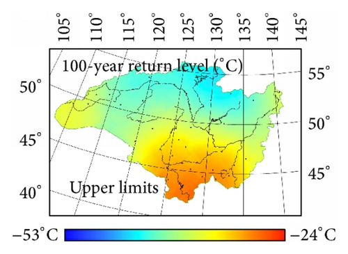
The increase in temperature intensity is a widespread phenomenon of global scale, and regional and local differences in magnitude and other characteristics also exist generally [8, 38]. For the extreme temperature of the Amur River basin, the local differences are very obvious. The increase in annual maximum temperature from observations at the 31 stations in central and northwest of the basin is consistent with the changes of the annual mean values, so is the increase in annual minimum temperature from observations at the 32 stations in the central basin. There are many reasons that could cause local differences, such as the latitude and altitude, the irregular topography, and the continental and marine climate. Particularly, researches on evaluating the impact of the Arctic Oscillation, the East Asian winter monsoon, Siberian High, and some factors of regional climate have been a popular trend [39–41], but it is not the point in our analyses, and detailed research on this issue can be considered in the future.

5. Conclusions

Climate changes for the annual mean and extreme temperature were detected by the M-K test, respectively. The annual mean temperature series increased significantly in whole basin, and the change points detected in all stations mostly occurred in 1980s. However, the changes of the extreme temperature presented obvious local differences compared with the mean value. The stations in Eastern and Northern basin had no change points for the annual maximum temperature, while other stations had change points that mainly occurred in 1990s, but not as concentrated as the mean value. Similarly, for the annual minimum temperature, there is no change point to be detected in 12 stations mainly located in Eastern and Northwestern basin. The change points of the other 32 stations occurred dispersedly. In addition, similarly to Novorotskii’s point of view [7], the increasing amplitude of the annual minima was greater than the annual maxima at the regional scale, while some individual stations presented local difference. The Northwestern stations had significant changes in annual maximum temperature, but no significant changes in annual minimum temperature.

Under climate change, the extreme climate events occurred frequently in Amur River basin, such as the heat wave in 2010 summer and the catastrophic floods in 2013. Estimating the accurate return levels for the extreme temperature was necessary. GVE distribution was used to fit the annual extreme temperature series in individual stations. The postchange point series was fitted in stations with change points, while the entire series was fitted in stations without change points. The regional spatial distribution of 10/50/100-year return levels presented the probability that occurrence of cold extremes in the central basin decreased, while the probability of occurrence of hot extremes in the central and Northwestern basin increased. It displayed a more severe situation and challenge for China and Russia to withstand extreme climate events and natural disaster together under climate change. Further work will focus on the relationship between extreme precipitation and extreme temperature and the potential impact of extreme weather on the river discharge, in order to provide references for the development of water resource in Amur River basin.

Competing Interests

The authors declare that there is no conflict of interests regarding the publication of this paper.

Acknowledgments

The current research is supported financially by the National Natural Science Foundation Projects of China (no. 41401011 and no. 41401010) and the Fundamental Research Funds for the Central Universities, China (nos. 2014B35514, 2014B20514, and 2015B03614).

References

1 Guo L. and Xia Z., Temperature and precipitation long-term trends and variations in the Ili-Balkhash Basin, Theoretical and Applied Climatology. (2014) 115, no. 1-2, 219–229, https://doi.org/10.1007/s00704-013-0883-3, 2-s2.0-84891661025.
10.1007/s00704-013-0883-3
Web of Science® Google Scholar
2 Huang F., Xia Z., Guo L., and Yang F., Climate change detection and annual extreme temperature analysis of the Irtysh Basin, Theoretical and Applied Climatology. (2013) 111, no. 3-4, 465–470, https://doi.org/10.1007/s00704-012-0676-0, 2-s2.0-84873166764.
10.1007/s00704-012-0676-0
Web of Science® Google Scholar
3 Pingale S. M., Khare D., Jat M. K., and Adamowski J., Spatial and temporal trends of mean and extreme rainfall and temperature for the 33 urban centers of the arid and semi-arid state of Rajasthan, India, Atmospheric Research. (2014) 138, 73–90, https://doi.org/10.1016/j.atmosres.2013.10.024, 2-s2.0-84888074899.
10.1016/j.atmosres.2013.10.024
Web of Science® Google Scholar
4 Starr J. R., Water wars, Foreign Policy. (1991) no. 82, 17–36, https://doi.org/10.2307/1148639.
10.2307/1148639
Google Scholar
5 Swain A., Managing Water Conflict: Asia, Africa and the Middle East, 2004, Routledge, London, UK.
10.4324/9780203502969
Google Scholar
6 Yu L.-L., Xia Z.-Q., Li J.-K., and Cai T., Climate change characteristics of Amur River, Water Science and Engineering. (2013) 6, no. 2, 131–144, https://doi.org/10.3882/j.issn.1674-2370.2013.02.002, 2-s2.0-84877271120.
10.3882/j.issn.1674-2370.2013.02.002
PubMed Google Scholar
7 Novorotskii P. V., Climate changes in the Amur River basin in the last 115 years, Russian Meteorology and Hydrology. (2007) 32, no. 2, 102–109, https://doi.org/10.3103/S1068373907020045, 2-s2.0-34548242225.
10.3103/S1068373907020045
Google Scholar
8 IPCC, T. F. Stocker, D. Qin, G.-K. Plattner et al., Summary for policymakers, Climate Change 2013: The Physical Science Basis: Working Group I Contribution to the Fifth Assessment Report of the Intergovernmental Panel on Climate Change, 2013, Cambridge University Press, Cambridge, UK, 3–29.
Google Scholar
9 Hansen J., Sato M., Ruedy R., Lo K., Lea D. W., and Medina-Elizade M., Global temperature change, Proceedings of the National Academy of Sciences of the United States of America. (2006) 103, no. 39, 14288–14293, https://doi.org/10.1073/pnas.0606291103, 2-s2.0-33749238010.
10.1073/pnas.0606291103
CAS PubMed Web of Science® Google Scholar
10 Aguilar E., Barry A. A., Brunet M., Ekang L., Fernandes A., Massoukina M., Mbah J., Mhanda A., do Nascimento D. J., Peterson T. C., Umba O. T., Tomou M., and Zhang X., Changes in temperature and precipitation extremes in western central Africa, Guinea Conakry, and Zimbabwe, 1955–2006, Journal of Geophysical Research: Atmospheres. (2009) 114, no. 2, D02115, https://doi.org/10.1029/2008jd011010, 2-s2.0-62849107372.
10.1029/2008JD011010
Web of Science® Google Scholar
11 Easterling D. R., Evans J. L., Groisman P. Y., Karl T. R., Kunkel K. E., and Ambenje P., Observed variability and trends in extreme climate events: a brief review, Bulletin of the American Meteorological Society. (2000) 81, no. 3, 417–425, https://doi.org/10.1175/1520-0477(2000)08160;0417:ovatie60;2.3.co;2, 2-s2.0-0001597306.
10.1175/1520-0477(2000)081<0417:OVATIE>2.3.CO;2
Web of Science® Google Scholar
12 Rusticucci M. and Tencer B., Observed changes in return values of annual temperature extremes over Argentina, Journal of Climate. (2008) 21, no. 21, 5455–5467, https://doi.org/10.1175/2008jcli2190.1, 2-s2.0-56349143827.
10.1175/2008JCLI2190.1
Web of Science® Google Scholar
13 Katz R. W. and Brown B. G., Extreme events in a changing climate: variability is more important than averages, Climatic Change. (1992) 21, no. 3, 289–302, https://doi.org/10.1007/bf00139728, 2-s2.0-2142722784.
10.1007/BF00139728
Web of Science® Google Scholar
14 Yang F., Sun Y., Yu T., Hou S., and Shen N., The spatiotemporal variation analysis of air temperature in heilongjiang province during 1997–2006, Journal of Geo-Information Science. (2009) 11, no. 5, 585–596, https://doi.org/10.3724/sp.j.1047.2009.00585.
10.3724/SP.J.1047.2009.00585
Google Scholar
15 Lu Z., Xia Z., Yu L., and Wang J., Characteristics of spatio-temporal variation of temperature in Songhua River Basin from 1960 to 2010, Journal of Hohai University (Natural Sciences). (2012) 40, no. 6, 629–635, https://doi.org/10.3876/j.issn.1000-1980.2012.06.006, 2-s2.0-84872451596.
10.3876/j.issn.1000-1980.2012.06.006
Google Scholar
16 Liu Y., Ruan H., Zhang P., and Li Y., Kriging interpolation of snow depthat the north of Tianshan Mountains assisted by MODIS data, Geomatics and Information Science of Wuhan University. (2012) 37, no. 4, 403–405, 2-s2.0-84860348705.
Google Scholar
17 Coles S., An Introduction to Statistical Modeling of Extreme Values, 2001, Springer, Springer Series in Statistics, https://doi.org/10.1007/978-1-4471-3675-0, MR1932132.
10.1007/978-1-4471-3675-0
Google Scholar
18 Makkonen L., Problems in the extreme value analysis, Structural Safety. (2008) 30, no. 5, 405–419, https://doi.org/10.1016/j.strusafe.2006.12.001, 2-s2.0-44449091448.
10.1016/j.strusafe.2006.12.001
Web of Science® Google Scholar
19 Leadbetter M. R., On a basis for ‘Peaks over Threshold’ modeling, Statistics & Probability Letters. (1991) 12, no. 4, 357–362, https://doi.org/10.1016/0167-7152(91)90107-3, 2-s2.0-0000014337.
10.1016/0167-7152(91)90107-3
Web of Science® Google Scholar
20 Bordi I., Fraedrich K., Petitta M., and Sutera A., Extreme value analysis of wet and dry periods in Sicily, Theoretical and Applied Climatology. (2007) 87, no. 1–4, 61–71, https://doi.org/10.1007/s00704-005-0195-3, 2-s2.0-33750493618.
10.1007/s00704-005-0195-3
Web of Science® Google Scholar
21 Burke E. J., Perry R. H. J., and Brown S. J., An extreme value analysis of UK drought and projections of change in the future, Journal of Hydrology. (2010) 388, no. 1-2, 131–143, https://doi.org/10.1016/j.jhydrol.2010.04.035, 2-s2.0-78149411575.
10.1016/j.jhydrol.2010.04.035
Web of Science® Google Scholar
22 Rusticucci M. and Tencer B., Observed changes in return values of annual temperature extremes over Argentina, Journal of Climate. (2008) 21, no. 21, 5455–5467, https://doi.org/10.1175/2008JCLI2190.1, 2-s2.0-56349143827.
10.1175/2008JCLI2190.1
Web of Science® Google Scholar
23 Kioutsioukis I., Melas D., and Zerefos C., Statistical assessment of changes in climate extremes over Greece (1955–2002), International Journal of Climatology. (2010) 30, no. 11, 1723–1737, https://doi.org/10.1002/joc.2030, 2-s2.0-77952929143.
10.1002/joc.2030
Web of Science® Google Scholar
24 Jeon S., Prabhat, Byna S., Gu J., Collins W. D., and Wehner M. F., Characterization of extreme precipitation within atmospheric river events over California, Advances in Statistical Climatology, Meteorology and Oceanography. (2015) 1, no. 1, 45–57, https://doi.org/10.5194/ascmo-1-45-2015.
10.5194/ascmo-1-45-2015
Google Scholar
25 Li Z., Li Z., Zhao W., and Wang Y., Probability modeling of precipitation extremes over two river basins in northwest of China, Advances in Meteorology. (2015) 2015, 13, 374127, https://doi.org/10.1155/2015/374127, 2-s2.0-84929378535.
10.1155/2015/374127
Web of Science® Google Scholar
26 Simonov E. A. and Dahmer T. D., Amur-Heilong River Basin Reader, 2008, Ecosystems.
Google Scholar
27 Wang X. L., Accounting for autocorrelation in detecting mean shifts in climate data series using the penalized maximal t or F test, Journal of Applied Meteorology and Climatology. (2008) 47, no. 9, 2423–2444, https://doi.org/10.1175/2008JAMC1741.1, 2-s2.0-45249103253.
10.1175/2008JAMC1741.1
Web of Science® Google Scholar
28 Wang X. L., Penalized maximal F test for detecting undocumented mean shift without trend change, Journal of Atmospheric and Oceanic Technology. (2008) 25, no. 3, 368–384, https://doi.org/10.1175/2007jtecha982.1, 2-s2.0-45249124469.
10.1175/2007JTECHA982.1
PubMed Web of Science® Google Scholar
29 Wu Q., Lang G., Wu Y., and Cang Y., Four seasons division and climate characteristic analysis of Heilongjiang province, Forest Investigation Design. (2009) 4, 95–96.
Google Scholar
30 Helsel D. R. and Hirsch R. M., Statistical Methods in Water Resources, 1992, Elsevier.
10.1016/S0166-1116(08)71099-9
Google Scholar
31 Mann H. B., Nonparametric tests against trend, Econometrica. (1945) 13, no. 3, 245–259, https://doi.org/10.2307/1907187, MR0012405.
10.2307/1907187
Web of Science® Google Scholar
32 Yin Y., Liu H., Yi X., and Liu W., Spatiotemporal variation and abrupt change analysis of temperature from 1960 to 2012 in the Huang-Huai-Hai Plain, China, Advances in Meteorology. (2015) 2015, 11, 643493, https://doi.org/10.1155/2015/643493, 2-s2.0-84929358924.
10.1155/2015/643493
Web of Science® Google Scholar
33 Carbone M., Turco M., Brunetti G., and Piro P., A cumulative rainfall function for subhourly design storm in Mediterranean Urban areas, Advances in Meteorology. (2015) 2015, 10, 528564, https://doi.org/10.1155/2015/528564, 2-s2.0-84938099065.
10.1155/2015/528564
Web of Science® Google Scholar
34 Panin G. N., Solomonova I. V., and Vyruchalkina T. Y., Climatic trends in the middle and high latitudes of the Northern Hemisphere, Water Resources. (2009) 36, no. 6, 718–730, https://doi.org/10.1134/S0097807809060116, 2-s2.0-70450174184.
10.1134/S0097807809060116
CAS Web of Science® Google Scholar
35 Pan H., Zhang G., and Xu N., A preliminary analysis of climate warming in Heilongjiang province since the 1980s, Climatic and Environmental Research. (2003) 8, no. 3, 348–355.
Google Scholar
36 Pan H. and Zhang G., Climate warner time-space variable features in Heilongjiang, Heilongjiang Meteorology. (2002) no. 3, 3–6.
Google Scholar
37 Sun F., Yang X., Lu S., and Yang S., The contrast analysis on the average and extremum temperature trend in Northeast China, Scientia Meteorologica Sinica. (2006) 26, no. 2, 157–163.
Google Scholar
38 Easterling D. R., Horton B., Jones P. D., Peterson T. C., Karl T. R., Parker D. E., Salinger M. J., Razuvayev V., Plummer N., Jamason P., and Folland C. K., Maximum and minimum temperature trends for the globe, Science. (1997) 277, no. 5324, 364–367, https://doi.org/10.1126/science.277.5324.364, 2-s2.0-9844226794.
10.1126/science.277.5324.364
CAS Web of Science® Google Scholar
39 Wu B. and Wang J., Winter arctic oscillation, Siberian High and East Asian winter monsoon, Geophysical Research Letters. (2002) 29, no. 19, 31–34, 2-s2.0-0036819969.
10.1029/2002GL015373
Web of Science® Google Scholar
40 Xiang L., Li X., Miu Q., Ma D., and Liu Z., Variation characteristics of temperature in Northeast China and relationships with sea-land pressure index at same latitude in recent 50 years, Journal of Anhui Agricultural Sciences. (2015) 43, no. 19, 190–194.
Google Scholar
41 Alessio S., Taricco C., Rubinetti S., Vivaldo G., and Mancuso S., Temperature and precipitation in Northeast China during the last 150 years: relationship to large-scale climatic variability, Annales Geophysicae. (2014) 32, no. 7, 749–760, https://doi.org/10.5194/angeo-32-749-2014, 2-s2.0-84903789071.
10.5194/angeo-32-749-2014
Web of Science® Google Scholar

Citing Literature

All articles

Climate Change Detection and Annual Extreme Temperature Analysis of the Amur River Basin

Abstract

1. Introduction