Volume 2016, Issue 1 2869083
Research Article
Open Access

Nonlinear Dynamics and Analysis of Intracranial Saccular Aneurysms with Growth and Remodeling

Manal Badgaish

Manal Badgaish

Department of Mathematical Sciences, George Mason University, Fairfax, VA 22030, USA gmu.edu

Search for more papers by this author
Jeng-Eng Lin

Jeng-Eng Lin

Department of Mathematical Sciences, George Mason University, Fairfax, VA 22030, USA gmu.edu

Search for more papers by this author
Padmanabhan Seshaiyer

Corresponding Author

Padmanabhan Seshaiyer

Department of Mathematical Sciences, George Mason University, Fairfax, VA 22030, USA gmu.edu

Search for more papers by this author
First published: 16 June 2016
Academic Editor: Giovanni P. Galdi

Abstract

A new mathematical model for the interaction of blood flow with the arterial wall surrounded by cerebral spinal fluid is developed with applications to intracranial saccular aneurysms. The blood pressure acting on the inner arterial wall is modeled via a Fourier series, the arterial wall is modeled as a spring-mass system incorporating growth and remodeling, and the surrounding cerebral spinal fluid is modeled via a simplified one-dimensional compressible Euler equation with inviscid flow and negligible nonlinear effects. The resulting nonlinear coupled fluid-structure interaction problem is analyzed and a perturbation technique is employed to derive the first-order approximation solution to the system. An analytical solution is also derived for the linearized version of the problem using Laplace transforms. The solutions are validated against related work from the literature and the results suggest the biological significance of the inclusion of the growth and remodeling effects on the rupture of intracranial aneurysms.

1. Introduction

Intracranial saccular aneurysm is a focal dilatation of the arterial wall that can be found in the circle of Willis which is a network of vessels at the base of the brain. The aneurysm which is a soft tissue interacts with a variety of flows including the blood as well as the cerebral spinal fluid. Based on the influence of various biomechanical factors, the growing aneurysm can potentially rupture that leads to either a neurological disorder or death. About 80% to 90% of ruptured aneurysms lead to death [1]. One of the invasive treatments for intracranial saccular aneurysms is to employ surgical procedures which may be associated with risk and death [2].

Over the last two decades, there have been several efforts to investigate the genesis of this disease and to develop a way for prediction of rupture through mathematical modeling [36]. Different groups of researchers had identified the elastodynamics of the arterial wall interaction with the blood flow to be the main reason for the rupture of an aneurysm [79]. A coupled fluid-structure model to understand the elastodynamics better was later studied more extensively [1013]. These models introduced mathematical models of increasing complexity for intracranial saccular aneurysms that described the coupled interaction between blood, arterial wall, and cerebral spinal fluid (CSF). In [11], the CSF was modeled using simplified Navier-Stokes equations, whereas the arterial wall structure was modeled using a spring-mass system. A Fourier series was used to model the interaction between blood pressure and inner wall. While the model developed yielded good insight into understanding rupture, this model did not accommodate growth and remodeling effects of the soft-tissue wall.

There are three main constituents of the artery wall, namely, the elastin, the collagen, and the smooth muscle [14, 15]. The elastin is a stable protein and is considered the most load bearing element that functions as resistance to the formation of an aneurysm, whereas the collagen is the protein that is responsible for preventing rupture after formation of an aneurysm. The growth of the aneurysm is associated with deficiency of elastin and weakening of the artery wall [16]. Hence, elastin and collagen should be incorporated into the modeling of arterial wall in order to obtain an accurate biological model of the aneurysm that maybe can lead to better interpretation and prediction for this disease. This is one of the main contributions of this work. In the model we will consider in this paper we will assume elastin and collagen to be one-dimensional passive fibers and also, for simplicity, we will not consider the effects of the smooth muscle for this work.

In Section 2, we will describe the mathematical model that we will consider to solve a coupled fluid-structure problem. Section 3 discusses the nonlinear analysis and perturbation solution for the model. In Section 4, the linearization of the growth and remodeling model is considered and solved analytically using Laplace transformation. After that, some important computational results and comparisons are discussed in Section 5. Finally, we conclude by some biological interpretation of the results and suggestion for future work.

2. Models and Background

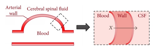
The mathematical modeling of intracranial saccular aneurysm builds on models developed in [11, 12] which included a simple mathematical model of a thin-walled, spherical intracranial aneurysm surrounded by cerebral spinal fluid which is referred to as CSF (see Figure 1).
Details are in the caption following the image
Model of an aneurysm in an arterial wall with blood inside and CSF outside.

The model was based on three separate components: modeling the blood pressure acting on the inner wall of the arteries, modeling the CSF that is located outside the wall, and modeling the arterial wall itself. Combining the various components yields a coupled fluid-structure interaction model. This model assumed a simple spring-mass model for the wall and the focus of this paper is to enhance this wall model to incorporate realistic nonlinear soft-tissue behavior.

2.1. Model of the Blood Pressure

The blood pressure is modeled using finite Fourier series since we consider the behavior to be pulsatile [10, 17, 18]:
()
where Pm is the mean blood pressure, w is the fundamental circular frequency, and An and Bn are the Fourier coefficients for N harmonic.

2.2. Model of the Arterial Wall

We consider the arterial wall to be modeled using a simple spring-mass system that incorporates the elastin and collagen effects in the outer wall of the arteries. The force of this system may be denoted by FS which is given by
()
where KE and  KC are the scaling coefficients, AE(t) and AC(t) are the cross-sectional areas, and σE(ϵE) and σC(ϵC) are the stresses for elastin and collagen, respectively. FS may be considered the force exerted on the outer wall. It is expressed in terms of the respective forces in the elastin and collagen along with the force from the blood pressure in the opposite direction. Each of the respective forces from the elastin and collagen is proportional to the respective stresses σE and σC. These forces help to balance the force expressed by the blood flow on the inner wall.
In this work we assume that these stresses are related to the respective strains through linear constitutive laws (material linearity) given by
()
and the strains are assumed to be nonlinear (geometric nonlinearity) given by
()
where L denotes the length of the unstrained tissue, u its extension, and r is the stretched factor of unstrained tissue of collagen fiber [6].

2.3. Model of the Cerebral Spinal Fluid

The model of CSF that is considered in this paper is the simplified one-dimensional compressible Euler equation with inviscid flow. Assuming negligible nonlinear effects and a constitutive relationship for the pressure [11], one can derive the following wave equation:
()
Here u(x, t) is assumed to be the displacement of the CSF with v(x, t) as the velocity. Since we are looking to find the movement of outer wall due to the interaction with CSF, we consider x = 0 to denote the outer wall and therefore we are interested in finding the solution to (5) at x = 0 that will describe the movement of the wall at any time t ≥ 0. In order to solve the system, we will assume that the displacement and velocity of the CSF is zero initially. This is given by the initial conditions:
()
The boundary conditions will be described later after the discussion of the modeling of the blood pressure and the arterial wall.

2.4. Governing Equation of Motion

In order to solve system (5), we need two boundary conditions. The first boundary condition is at point x = 0, and it can be derived from the model of blood pressure and the arterial wall that we have discussed. Note that the force balance equation at x = 0 may be written as
()
Here,
()
is the total force, where m is the mass of the wall. Consider that
()
is the force of the fluid which is the product of the pressure P and the cross-sectional area a. The pressure is given by P = −ρc2ux, where ρ is the density of the CSF which is assumed to be slightly compressible [11]. The total force of the spring from (2) is given by
()
Then, substituting (8), (9), and (10) into (7) we obtain the first boundary condition at x = 0:
()
The second boundary condition can be obtained using the plane wave approximation that states that the waves from the wall will die down some fixed distance away from the wall. If this can be applied at point x = L, then the second boundary condition becomes [11]
()
Combining (5), (6), (11), and (12), we obtain the following coupled fluid-structure interaction problem:
()
Solving the above coupled system will yield u(x, t) which is the displacement of the fluid in the domain [0, L]. Note that the displacement of the outer boundary of the wall is the same as u(0, t) which is the displacement of the fluid at the left end boundary of its domain. As described in [11], we will also study the movement of the outer wall, namely, u(0, t), to be an indicator of the potential for rupture of the aneurysm. The higher the value of u(0, t), the more the potential for rupture. However, one must solve nonlinear coupled system (13) which does not admit an exact solution. One must therefore apply other approaches to obtain this solution. Next, we will employ a nonlinear analysis and perturbation method in this model to obtain an approximate solution to system (13) which is one of the central contributions of this work.

3. Nonlinear Dynamics and Analysis

Nonlinear analysis and perturbation method techniques are powerful tools to study the behavior of complex nonlinear models and help to obtain an approximate solution to these models. In this work, the nonlinear phase analysis and perturbation technique for (13) will be presented. We will employ the following steps. First we will convert (13) which is an initial-boundary value partial differential equation system into an initial value ordinary differential equation system. Following this we will perform a phase analysis of the newly obtained initial value differential equation. We will then apply the perturbation techniques to the resulting equations. These steps are described next.

3.1. Converting the PDE System into Initial Value Differential Equation

Since the governing equation of system (13) is a one-dimensional wave equation, it has a unique solution of the form [19]
()
Differentiating the above solution with respect to variables x and t yields
()
()
()
()
Substituting (15)–(17) in the boundary condition at x = L of system (13) yields
()
This yields and therefore
()
where D is arbitrary constant. Using (14), the unique solution of the wave equation becomes
()
Since D is an arbitrary constant, it can be absorbed inside the function . Therefore, the general solution of the system is
()
Since our goal is to determine the solution u(0, t), next we substitute (22) into the boundary condition at x = 0 of system (13) which yields
()
which can be rewritten as
()
with the following initial condition: f(0) = 0, f(0) = 0. Here,
()

Lemma 1. Nonlinear differential equation (24) can be rewritten as the following nonlinear second-order differential equation:

()

Proof. To prove this, we will use a change of variable. Let us define T = −ct and substitute this in differential equation (24) to obtain  

()
Next, we will choose another change of variable and let . Also define a new function . Then applying chain rule, we have
()
Using these relations and renaming , (27) can be rewritten as
()
Note that the last summation term in (29) is now 2π periodic.

3.2. Phase Analysis of the Initial Value Differential Equation
Consider the homogeneous case for (29). Dividing throughout by mw2 yields
()
where
()
Defining a new vector,
()
where and ; we can now rewrite (30) into two first-order equations as follows:
()
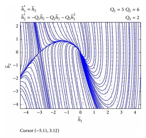
It is trivial to note from the system above that there are two equilibrium points, namely, the origin (0,0) and the point (−Q2/Q3, 0).
Considering the first equilibrium point, that is (0,0), system (33) can be rewritten in a matrix form as
()
where
()
The linearized part of (34) is
()
The eigenvalues of the matrix A are two negative real numbers that can be calculated using
()
and since none of the eigenvalues of A has zero real part, the equilibrium point is hyperbolic. Hence, the behavior of nonlinear system (34) is topologically equivalent to the behavior of linearized system (36), and the approximate solution for this linear system will be good first approximation for nonlinear system (34) [20]. Note that we will restrict the values of ρ,  c,  a,  m,  w,  KE,  KC,  AE,  AC,  L, and r in order to have two distinct real eigenvalues. This means that
()
This condition as we will see later has biological significance in relation to the displacement of the outer wall. Analyzing the behavior of linear system, it can be seen that the origin (0,0) is a stable node (sink) for linear system (36). Thus, it is a stable node for nonlinear system (34) as well [20]. Therefore, in area around the origin the solution is supposed to approach the equilibrium point (see Figure 2).
Details are in the caption following the image
Phase portrait of the system.
In order to study the behavior of the nonlinear solution near the second equilibrium point, that is (−Q2/Q3, 0), this equilibrium point has to be translated to the origin using the following transformation:
()
Using above transformation, the new system can be rewritten as
()
This can be written in matrix form as
()
where
()
The linearized part of (41) is
()
The eigenvalues of the matrix are two distinct real numbers with opposite signs and can be calculated using
()
Therefore, the behavior of nonlinear system (41) is topologically equivalent to the behavior of linearized system (43). We have found that this equilibrium point (−Q2/Q3, 0) is unstable saddle for the linear system; therefore, it is also an unstable saddle for the nonlinear system [20].

3.3. Existence of the Solution to Perturbed Nonlinear Nonhomogeneous System

Let us consider again the following second-order nonhomogeneous weakly nonlinear ODE:
()
where
()
is 2π periodic Fourier series and Q4 = 1/mw2. This system can be written in vector form as
()
where and .
The associated reduced system when ϵ = 0 is
()
A particular solution of reduced system (48) is expressed as
()
where
()
Note that, from here, we can obtain all the general solutions for (48) which will require the application of the initial conditions to solve for any unknown constants in the general solution. Then, (45) has a 2π periodic solution h = h(t, ϵ) that is analytic in ϵ. Therefore, the solution can be expressed as convergent power series [21]:
()
where each function hn(t) is 2π periodic in t.

3.4. Perturbation Technique to Find First-Order Approximation

Let us consider (24) with perturbed term:
()
with the following initial condition: f(0) = 0, f(0) = 0, where
()
and ϵ here is assumed to be very small. Following the ideas in Lemma 1, the above differential equation can be rewritten as
()
with h(0) = 0,   h(0) = 0. Let the solution of differential equation (54) be expressed as power series as in the previous section. Replacing the function h(t) by its power series (51) and comparing coefficients of each order, we obtain the following [2224].
Zeroth-Order Approximation. Consider
()
First-Order Approximation. Consider
()
We can now solve (55) that yields
()
where
()
Since we have restriction condition from Section 3.2, that is, , this is identical to the following condition:
()
Hence, λ1λ2.
Using solution h0(t) from (57), we can rewrite (56) in the form
()
Solution to (60) can be derived to be
()
where
()
where
()
For simplicity, we restricted the solution to be first-order approximation, so
()
and then we can have a first-order approximation of the solution we are looking for which is given by
()
where h0 and  h1 are defined in (57) and (61), respectively.

4. Linearization of the Growth and Remodeling Model

Since the growth and remodeling model discussed in the previous section is a nonlinear model that does not admit an exact solution, it would be be beneficial to consider the linearized version of this model and solve it analytically using Laplace transform. The linearization can be done using Taylor series expansion of the nonlinear terms in the boundary condition in (13) to yield
()
()
()
()
To obtain the exact solution to this linearized system, we will consider the Laplace transform of PDE (66) which becomes
()
The solution to (70) can be easily shown to be
()
Taking the Laplace transform of boundary conditions (68)-(69), we obtain
()
()
In order to find the constants C1 and C2, we substitute (71) into (73) and compare the coefficient which yields
()
Since we are interested in solution to displacement of cerebral spinal fluid (CSF) at x = 0, we take Laplace transform of boundary condition at x = 0 (72) and then substitute the solution (71) into it to obtain
()
Taking the inverse of Laplace transformation will give us the solution of the displacement of the CSF at x = 0 which is given by
()
where
()
Equation (76) above represents a solution to the linearized model for the movement of the outer wall for all time t ≥ 0. Obviously, the solution is the summation of exponential terms, constant terms, and periodic terms. The form of the solution suggests that the solution should start from the origin since the given initial condition is u(0,0) = f(0) = 0. It is well known that the constant and periodic terms are bounded. Hence, the exponential term should be analyzed in order to understand the behavior of solution (76).
The exponential terms in above solution (76) are in the forms eλt, and note that, in order for r1,2 to be real and distinct, we will restrict the values of ρ,  c,  a,  m,  KE,  KC,  AE,  AC,  L, and r. Hence, we need
()
Furthermore, from the given data for the problem and since all the constants in r1,2 are positive, we found that both values of r1,2 are negative. Therefore, the exponential terms will act in the first few time steps only and they will go to zero as t becomes large. In this case, the periodic terms and the constant will be dominant as t approaches infinity. This decay may be considered biologically significant in the displacement of the outer wall which relates to the rupture of the aneurysm.

5. Computational Experiments

In this section we perform numerical studies that will help to validate the theory presented in this work. For our computational experiments, the following realistic values are utilized. For the CSF, ρ = 1000 kg/m3 and c = 1500 m/s are used. For the wall, a = 0.01 m2, KE = 800 N/m, KC = 3.52 N/m, AE = 20 m2, AC = 10 m2, r = 2 m, m = 0.001 kg, and L = 1.5 m are used. Finally, Pm = 8759.279403 mmHg and w = 1 rad/s are used for the blood pressure model, and, for the harmonics, A1 = −7.13, A2 = −3.08, A3 = −0.130, A4 = −0.205, A5 = 0.0662, B1 = 4.64, B2 = −1.18, B3 = −0.564,  and B4 = −0.346, B5 = −0.120, all in mmHg [11]. Note that these values meet both restrictions (59) and (78), respectively. For example, (78) can be verified as follows:
()
Similarly (59) can also be verified.

5.1. Validation of the Perturbation Solution

First, we compare the first-order solution obtained in (65) using perturbation analysis against the linearized growth and remodeling model solution obtained analytically using Laplace transform in (76). In Figure 3, we plot these two solutions against the solution obtained from the linear model previously obtained by [11].

Details are in the caption following the image
Validation of the perturbation solution for the growth and remodeling model.

First, it is interesting to note that the solution to the linearized problem with growth and remodeling obtained via Laplace transform is close to the solution for nonlinear growth and remodeling problem obtained via perturbation method. The figure also illustrates that solution for the nonlinear problem obtained via the perturbation approach also has the same behavior but differs from the solution from [11]. This goes to show that the growth and remodeling effects are important and have a significant influence on the model. Moreover, the growth and remodeling model has the effect of reducing the displacement of the outer wall and preventing the aneurysm rupture consequently. In order to understand this further, we investigate the influence of elastin and collagen contributions in the growth and remodeling process on the potential of rupture. This is discussed next.

5.2. Influence of Collagen and Elastin Parameters

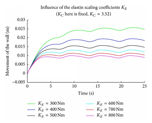
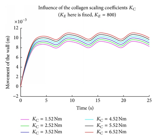
The elastic and collagen parameters (KE, KC) seem to play an important role in the modeling of the arterial wall since they are responsible for the elasticity and strength of wall tissue. It is known from the literature that a deficiency in elastin and an increase in collagen are often related to the rupture of an aneurysm. Figure 4 shows the solution of the nonlinear coupled problem using the perturbation solution for increasing values of KE starting from 800 N/M till 300 N/M. This corresponds to simulating the effect of deficiency in elastin and the figure clearly illustrates that as the KE value decreases the displacement of the outer wall increases which can lead to rupture. Figure 5 shows that the displacement of the outer wall increases in a steady periodic motion as KC increases which suggests biologically that an increase in collagen may lead to rupture. These findings are consistent with experimental findings which suggest the robustness of the one-dimensional model considered in this paper.
Details are in the caption following the image
Influence of elastin scaling coefficient.
Details are in the caption following the image
Influence of collagen scaling coefficient.

6. Conclusion and Future Work

In this work a new mathematical model was considered that couples the elastodynamics of the blood coupled with the arterial wall dynamics and the mechanics of cerebral spinal fluid. This geometrically nonlinear coupled fluid-structure problem for the first time considered the effects of growth and remodeling and a phase analysis of the model was presented. Since this nonlinear system does not admit an exact solution, the model was analyzed using perturbation techniques to obtain approximate solutions. Section 3 discusses the nonlinear analysis and perturbation solution for the model. The nonlinear coupled system was also linearized and a Laplace transform method was applied to derive the exact solution to the linearized problem. The models proposed in this paper compares well with similar models published for the linear case. Our results also seem to justify what has been experimentally observed by other research groups regarding the rupture of an aneurysm in relation to a deficiency in elastin and/or an increase in collagen. The novelty of the current paper is in the formulation, analysis, and simulation of the nonlinear coupled fluid-structure interaction model that incorporates growth and remodeling. The results from the computational experiments presented give encouragement to the authors to incorporate more features into the existing model such as incorporating viscoelasticity of the wall, adding nonlinear effects in the fluid model, and obtaining a fully implicit numerical approximation to the solution. These aspects will be considered in forthcoming papers.

Competing Interests

The authors declare that they have no competing interests.

    The full text of this article hosted at iucr.org is unavailable due to technical difficulties.