Volume 2016, Issue 1 2741891
Research Article
Open Access

Qualitative Analysis of a Leslie-Gower Predator-Prey System with Nonlinear Harvesting in Predator

Manoj Kumar Singh

Corresponding Author

Manoj Kumar Singh

Department of Applied Mathematics, School for Physical Sciences, Babasaheb Bhimrao Ambedkar University, Lucknow 226025, India bbau.ac.in

Search for more papers by this author
B. S. Bhadauria

B. S. Bhadauria

Department of Applied Mathematics, School for Physical Sciences, Babasaheb Bhimrao Ambedkar University, Lucknow 226025, India bbau.ac.in

Department of Mathematics, Faculty of Sciences, Banaras Hindu University, Varanasi 221605, India bhu.ac.in

Search for more papers by this author
Brajesh Kumar Singh

Brajesh Kumar Singh

Department of Applied Mathematics, School for Physical Sciences, Babasaheb Bhimrao Ambedkar University, Lucknow 226025, India bbau.ac.in

Search for more papers by this author
First published: 03 October 2016
Citations: 6
Academic Editor: Krishnan Balachandran

Abstract

This paper deals with the study of the stability and the bifurcation analysis of a Leslie-Gower predator-prey model with Michaelis-Menten type predator harvesting. It is shown that the proposed model exhibits the bistability for certain parametric conditions. Dulac’s criterion has been adopted to obtain the sufficient conditions for the global stability of the model. Moreover, the model exhibits different kinds of bifurcations (e.g., the saddle-node bifurcation, the subcritical and supercritical Hopf bifurcations, Bogdanov-Takens bifurcation, and the homoclinic bifurcation) whenever the values of parameters of the model vary. The analytical findings and numerical simulations reveal far richer and complex dynamics in comparison to the models with no harvesting and with constant-yield predator harvesting.

1. Introduction

Marine life is a renewable natural resource that not only provides food to a large population of humans but also is involved in the regulation of the Earth’s ecosystem. The growing human needs for more food and more energy have led to increased exploitation of these resources which affects the Earth’s ecosystem. Thus, it is imperative to design harvesting strategies which aim at maximizing economic gains giving due consideration to the ecological health of the concerned Earth’s ecological system. Mathematical modeling in harvesting of species was started by Clark [1, 2]. There are mainly three types of harvesting according to Gupta et al. [3]: (i) h(x) = h, constant rate harvesting (see [47]), (ii) h(x) = qEx, proportionate harvesting (see [8, 9]), and (iii) h(x) = qEx/(m1E + m2x) (Holling type II), nonlinear harvesting (see [1013]). Nonlinear harvesting is more realistic and exhibits saturation effects with respect to both the stock abundance and the effort level. Notice that h(x) → qE/m2 as x and h(x) → qE/m1 as E.

The objective of the present work is to study dynamical behaviors of a Leslie-Gower predator-prey model in the presence of nonlinear harvesting in predators depending on parameters of the model. There have been many papers on the Leslie-Gower predator-prey system with harvesting. For example, May et al. [14] proposed a Leslie-Gower predator-prey model in which two different kinds of constant-yield harvesting applied on both prey and predator species have been considered and this model was studied by Beddington and Cooke [15]. Beddington and May [16] proposed and studied Leslie-Gower predator-prey model when both the prey and predators were harvested with constant effort. Beddington and Cooke [15] studied a Leslie-Gower predator-prey model in which the preys are harvested at a constant-yield rate and predators are harvested with constant-effort rate. Zhu and Lan [17] studied a Leslie-Gower predator-prey model with constant-yield prey harvesting. Gong and Huang [18] studied the Bogdanov-Takens bifurcation for the model and showed that for different parameter values the model has a limit cycle or a homoclinic loop. Gupta et al. [3] discussed the bifurcation analysis of a Leslie-Gower prey-predator model in the presence of nonlinear harvesting in prey. Huang et al. [19] studied the effect of constant-yield predator harvesting on the dynamics of a Leslie-Gower type model and showed that the model has Bogdanov-Takens (BT) singularity of codimension 3 or a weak focus of multiplicity two for some parameter values. They have shown that as the parameters change, the model exhibits saddle-node bifurcation, repelling and attracting B-T bifurcations, and supercritical, subcritical, and degenerate Hopf bifurcations.

This article is organized as follows. In Section 2, we describe the mathematical model in detail. In Section 3, we obtain the number and location of equilibrium points and the local and global stability of the equilibria are investigated. In Section 4, the existence of saddle-node, Hopf, and Bogdanov-Takens bifurcations is shown. In Section 5, we present several numerical simulations that support our theoretical results. Finally, we present some ramification of our results in Section 6.

2. Model Equations

2.1. Leslie-Gower Model

In general, the Leslie-Gower predator-prey model [20] is given as follows:
()
where XX(T) and YY(T) are the prey density and predator density at time T, respectively; r, s, K, m, and n are positive parameters and represent the intrinsic growth rate of prey, intrinsic growth rate of predator, carrying capacity of prey in the absence of predator, maximal predator per capita consumption rate, and measure of the food quality that the prey provides for conversion into predator births. Model (1) has been studied by Hsu and Huang [21]. They showed that the unique positive interior equilibrium point of system (1) is globally asymptotically stable under all biologically admissible parameters.

2.2. Harvested Model

We assumed that only predator species is economically important and the nonlinear harvesting rate is considered. Model (1) reduces to the following:
()
where the parameters q and E are positive and represent catchability coefficient and effort applied to harvest the individuals, respectively, and m1,   m2 are suitable positive constants.
Model (2) is not well defined at (0,0). In order to define system (2) at (0,0), we improve the model as given in [22]; system (2) reduces to
()
For nondimensionalizing system (3), we introduce the following substitutions:
()
System (3) reduces to
()
where ρ = s/r, β = r/mnK, h = qEm/srm2, and c = m1mE/m2r. For the existence of the biological meaning of the variables in model, system (5) is studied in the closed first quadrant, Ω, in xy-plane defined by Ω = {(x, y):  x ≥ 0,   y ≥ 0}.

3. Equilibria and Their Local Stability

The equilibrium points of system (5) are the nonnegative real solutions of the system dx/dt = dy/dt = 0. It is obvious that system (5) has the trivial equilibrium point E0 = (0,0) and the axial equilibrium point e = (1,0) and the abscissa of the positive interior equilibrium points are the roots of the quadratic equation:
()
and the ordinance of the positive interior equilibrium points is given by y1,2 = 1 − x1,2, 0 ≤ x1,2 ≤ 1.

The quadratic equation (6) has two positive roots and whenever (say), a double positive root x3 = (1 + 2β + c + βch)/2(1 + β) whenever , and no positive root whenever . The number and location of the equilibrium points of system (5) lying in the set Ω are given in the following lemma.

Lemma 1. System (5) has

  • (a)

    four equilibrium points, trivial equilibrium point E0 = (0,0), axial equilibrium point e = (1,0), and two interior equilibrium points E1 = (x1, y1) and E2 = (x2, y2) whenever , where , , , , and ;

  • (b)

    three equilibrium points, trivial equilibrium point E0 = (0,0), axial equilibrium point e = (1,0), and a double interior equilibrium point E3 = (x3, y3) whenever , where and ;

  • (c)

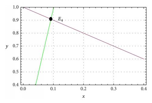
    three equilibrium points, trivial equilibrium point E0 = (0,0), axial equilibrium point e = (1,0), and an interior equilibrium point E4 = (x4, y4) whenever c = h and βc < 1, where x4 = β(1 + c)/(1 + β) and y4 = (1 − βc)/(1 + β);

  • (d)

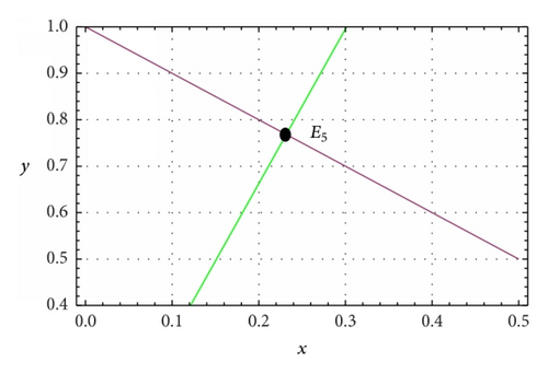
    three equilibrium points, trivial equilibrium point E0 = (0,0), axial equilibrium point e = (1,0), and an interior equilibrium point E5 = (x5, y5) whenever h < c, where and ;

  • (e)

    two equilibrium points, trivial equilibrium point E0 = (0,0), and axial equilibrium point e = (1,0) whenever and c < h.

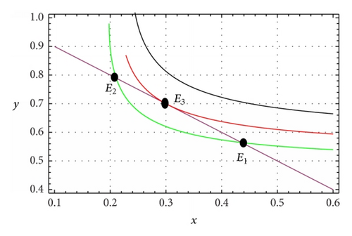
The number and location of interior equilibrium points have been depicted in Figure 1.
Details are in the caption following the image
This diagram shows the number and location of the positive interior equilibrium points of system (5). The green, red, and black color curves are the predator nullclines for different values of h and the straight line is the prey nullcline: (a) h > c, for black color parabola , for red color parabola , and for green color parabola ; (b) h = c; (c) h < c.
Now, we shall discuss the stability of the equilibrium points. The Jacobian matrix of system (5) at the equilibrium point E0 cannot be calculated as the term y/x is not defined at (0,0). We use the blow-up technique to analyze the stability of the equilibrium point E0 as given in [23]. Let x = x and y = xv; then, system (5) reduces to
()
System (7) has two equilibrium points and whenever ρ − 1 − hρ/c > 0. The Jacobian matrix of system (7) at the equilibrium point is
()
Thus, the equilibrium point of system (7) is an unstable point as ρ − 1 − hρ/c > 0. The Jacobian matrix of system (7) at the equilibrium point is
()
Thus, the equilibrium point of system (7) is always saddle as ρ − 1 − hρ/c > 0. Thus, we can conclude the discussion above as follows.

Theorem 2. The trivial equilibrium point E0 of system (5) is a saddle point.

The Jacobian matrix of system (5) at the equilibrium point e is
()
The Jacobian matrix of system (5) at the positive interior equilibrium point E is
()
The determinant of the abovementioned Jacobian matrix det⁡(JE) = (ρy/x(c + y))(β(1 + c)−(1 + β)x2) and trace tr⁡(JE) = (ρy/x)((x − 2βyβc)/(c + y)) − x.

Theorem 3. (a) The equilibrium point e is asymptotically stable whenever c < h and a saddle whenever h < c.

(b) The equilibrium point E1, if existent, is always a saddle point.

(c) The equilibrium point E2, if existent, is asymptotically stable whenever (ρy2/x2)((x2 − 2βy2βc)/(c + y2)) − x2 < 0 and is unstable whenever (ρy2/x2)((x2 − 2βy2βc)/(c + y2)) − x2 > 0.

(d) The equilibrium point E3, if existent, is a degenerate singular point.

(e) The equilibrium point E4, if existent, is always asymptotically stable.

(f) The equilibrium point E5, if existent, is asymptotically stable whenever (ρy5/x5)((x5 − 2βy5βc)/(c + y5)) − x5 < 0 and is unstable whenever (ρy5/x5)((x5 − 2βy5βc)/(c + y5)) − x5 > 0.

Proof. (a) The eigenvalues of the Jacobian matrix Je are −1 and ρ(1 − h/c), so the equilibrium point e is asymptotically stable whenever c < h and a saddle whenever h < c.

(b) The determinant , so the interior equilibrium point E1 is a saddle point.

(c) The determinant and , so the interior equilibrium point E2 is asymptotically stable whenever (ρy2/x2)((x2 − 2βy2βc)/(c + y2)) − x2 < 0 and unstable whenever (ρy2/x2)((x2 − 2βy2βc)/(c + y2)) − x2 > 0.

(d) The determinant , so the interior equilibrium point E3 is a degenerate singular point.

(e) The determinant as βc < 1 and always, so the interior equilibrium point E4 is always asymptotically stable.

(f) The determinant and , so the interior equilibrium point E5 is asymptotically stable whenever (ρy5/x5)((x5 − 2βy5βc)/(c + y5)) − x5 < 0 and unstable whenever (ρy5/x5)((x5 − 2βy5βc)/(c + y5)) − x5 > 0.

From Lemma 1, if h = c, system (5) has unique interior equilibrium point E4, and if h < c, system (5) has unique interior equilibrium point E5. In Theorem 3, it is proved that these interior equilibrium points are always asymptotically stable. Now we show that these equilibrium points are globally asymptotically stable.

Theorem 4. The equilibrium points E4 and E5, if existent, are globally asymptotically stable.

Proof. From Lemma 1, system (5) has one trivial equilibrium point E0, one axial equilibrium point e, and one interior equilibrium point E4 whenever h = c. Further, it has one trivial equilibrium point E0, one axial equilibrium point e, and one interior equilibrium point E5 whenever h < c. Also, from Theorem 3, the trivial equilibrium point E0 is always a saddle point, axial equilibrium point e is a saddle point whenever hc, and the interior equilibrium points E4 and E5 are asymptotically stable. We define the following function:

()
where f(x, y) = x(1 − xy), g(x, y) = ρy(1 − βy/xh/(c + y)), and M(x, y) = 1/xy2.

After simplification, we obtain L(x, y) = −(1/y2)(1 + (y2 + (ch)(c + 2y))/x(c + y) 2) < 0 as h = c or h < c. Thus, by using Dulac’s criterion [24], system (5) will not have any nontrivial periodic orbit in Ω. Note that y-axis and x-axis are the stable manifolds of the trivial and the axial equilibrium points, respectively. Using this in conjunction with the Poincare-Bendixson theorem [24] gives us that the interior equilibrium points E4 and E5 will be globally stable.

In Theorem 3, it is shown that the equilibrium point E3 is a degenerate singular point. Now we study the property of this point.

Theorem 5. The equilibrium point E3, if existent, is

  • (a)

    a saddle-node whenever (ρy3/x3)((x3 − 2βy3βc)/(c + y3)) − x3 ≠ 0;

  • (b)

    a cusp of codimension 2 whenever (ρy3/x3)((x3 − 2βy3βc)/(c + y3)) − x3 = 0.

Proof. First, we shall shift the equilibrium point E3 = (x3, y3) to the origin by using the transformations u1 = xx3 and v1 = yy3; system (5) reduces into the form

()
where
()
If (ρy3/x3)((x3 − 2βy3βc)/(c + y3)) − x3 ≠ 0, point E3 is a saddle point. Now we consider (ρy3/x3)((x3 − 2βy3βc)/(c + y3)) − x3 = 0; that is, . Both eigenvalues of the Jacobian matrix are zero and system (13) reduces to
()
Now we introduce the affine transformations u2 = u1, v2 = −x3u1x3v1, to reduce system (15) as
()
where
()
Now, we consider the C change of coordinates in the small vicinity of (0,0):
()
Then, system (16) reduces to
()
Now, we choose the C change of coordinates in the small neighbourhood of (0,0):
()
System (19) reduces to
()
Now, we choose the final C change of coordinates in the small neighbourhood of (0,0):
()
System (21) reduces to
()
If (nondegeneracy condition), the origin (0,0) of (23) is a cusp of codimension 2; that is, the interior equilibrium point E3 of system (5) is a cusp of codimension 2.

In Section 4, we shall study the bifurcations occurring in system (5).

4. Bifurcation Analysis

4.1. Hopf Bifurcation

In Theorem 3, it is shown that the interior equilibrium point E2 is stable whenever (ρy2/x2)((x2 − 2βy2βc)/(c + y2)) − x2 < 0 and unstable whenever (ρy2/x2)((x2 − 2βy2βc)/(c + y2)) − x2 > 0. Now, we consider the parametric condition (ρy2/x2)((x2 − 2βy2βc)/(c + y2)) − x2 = 0. In this parametric condition, the equilibrium point E2 is a weak focus or a center. Hence, system (5) may enter a Hopf bifurcation at the point E2. In this subsection, we consider the parameter ρ as the Hopf bifurcation parameter and discuss the conditions under which the stability of E2 will change and system (5) exhibits Hopf bifurcations.

Theorem 6. System (5) undergoes a Hopf bifurcation with respect to parameter ρ around the equilibrium point E2, if existent, whenever (ρy2/x2)((x2 − 2βy2βc)/(c + y2)) − x2 = 0. Moreover,

  • (a)

    the equilibrium point E2 is a weak focus of multiplicity 1 if the parameter set (ρ, β, h, c) is in Hsup or Hsub and is stable and unstable according to whether (ρ, β, h, c) is in Hsup or Hsub;

  • (b)

    system (5) has at least one unstable limit cycle whenever (ρ, β, h, c) is in Hsub,   0 < ρ < ρ and |ρρ| ≪ 1, and at least one stable limit cycle whenever (ρ, β, h, c) is in Hsup,   ρ > ρ and |ρρ| ≪ 1.

Proof. A critical magnitude of the bifurcation parameter exists as 1 − βc − (1 + 2β)y2 ≠ 0 such that, at ρ = ρ, tr⁡(JE) = 0 and det⁡(JE) > 0. In order to ensure the existence of a Hopf bifurcation, we have to check the transversality condition (see [24]). We have as 1 − βc − (1 + 2β)y2 ≠ 0. Hence, the transversality condition for a Hopf bifurcation is satisfied. To determine the direction of Hopf bifurcation and stability of E2, we compute the first Liapunov coefficient of system (5) at the equilibrium point E2.

Let x = ux2 and y = vy2; then, the equilibrium point E2 is shifted to the origin (0,0) and system (5) can be rewritten as

()
where a10 = −x2, a01 = −x2, a20 = −1, a11 = −1, a02 = 0, a30 = 0,   a21 = 0, a12 = 0, a03 = 0, , b01 = (ρy2/x2)((x2βy2)/(c + y2) − β), , , b02 = ρ(ch/(c + y2) 3β/x2), , b12 = ρβ/x2, b03 = ρy2h/(c + y2) 4βh/(c + y2) 3, and . Hence, using the formula of the first Lyapunov number σ at the origin of (24), we have
()
where . If σ ≠ 0, then the origin of (24) is a weak focus of multiplicity one: also origin is stable when σ < 0 and unstable when σ > 0. Hence, in parameter space (ρ, β, h, c), there exist surfaces and , called subcritical and supercritical Hopf bifurcation surface, respectively, such that if the parameter set (ρ, β, h, c) is in Hsub, the equilibrium point E2 of system (5) is a weak focus of multiplicity 1 and is unstable, and if the parameter set (ρ, β, h, c) is in Hsup, the equilibrium point E2 of system (5) is a weak focus of multiplicity 1 and is stable.

From the discussion above, the equilibrium point E2 of system (5) is a weak focus of multiplicity 1 and is unstable if (ρ, β, h, c) is in Hsub. Also from Theorem 3, the equilibrium point E2 is stable whenever (ρy2/x2)((x2βy2)/(c + y2) − β) − x2 < 0, that is, ρ < ρ, and is unstable whenever (ρy2/x2)((x2βy2)/(c + y2) − β) − x2 > 0, that is, ρ > ρ. Thus, the equilibrium point E2 generates an unstable limit cycle as the bifurcation parameter ρ passes through the bifurcation value ρ = ρ. From one side of the surface Hsub to the other side, system (5) can undergo a subcritical Hopf bifurcation. An unstable limit cycle arises in the small neighbourhood of the equilibrium point E2 whenever (ρ, β, h, c) is in Hsub,   0 < ρ < ρ and |ρρ| ≪ 1. Similarly, a stable limit cycle arises in the small neighbourhood of the equilibrium point E2 whenever (ρ, β, h, c) is in Hsup,   ρ > ρ and |ρρ| ≪ 1.

4.2. Saddle-Node Bifurcation

In Section 3, it is shown that system (5) admits the double point E3 whenever . In Theorem 5, it is shown that the point E3 is a saddle node whenever (ρy3/x3)((x3 − 2βy3βc)/(c + y3)) − x3 ≠ 0. Now, we show that system (5) experiences a saddle-node bifurcation of codimension 1 around the equilibrium point E3 at the threshold value of the bifurcation parameter by means of Sotomayor’s theorem [24].

Theorem 7. System (5) undergoes a saddle-node bifurcation with respect to the parameter h around the equilibrium point E3 whenever and (ρy3/x3)((x3 − 2βy3βc)/(c + y3)) − x3 ≠ 0.

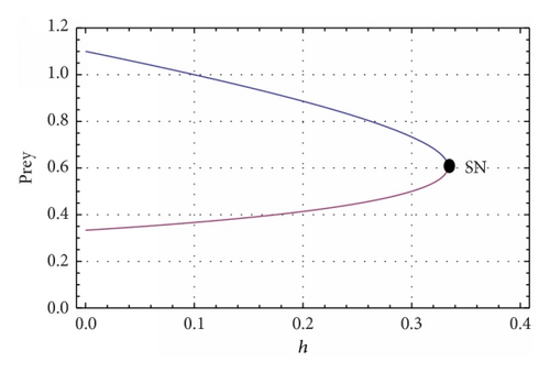
Proof. It has been shown that if and (ρy3/x3)((x3 − 2βy3βc)/(c + y3)) − x3 ≠ 0, one eigenvalue of the Jacobian matrix is zero and the other has nonzero real part. Suppose V and W are the eigenvectors corresponding to the zero eigenvalues of the Jacobian matrix and transpose matrix , respectively; then, and . We have , . Therefore, and . Since , . Thus, Sotomayor’s theorem confirms that system (5) experiences a saddle-node bifurcation of codimension 1 around interior equilibrium point E3. This means that there are no equilibrium points for while there are two coexistence equilibrium points E1 and E2 for , one of which is saddle point and the other is a stable node.

4.3. Bogdanov-Takens Bifurcation

In Theorem 5, we have proved that the interior equilibrium point E3 is a cusp of codimension 2 whenever (ρy3/x3)((x3 − 2βy3βc)/(c + y3)) − x3 = 0 and η4η5 ≠ 0, which implies that there may exist the Bogdanov-Takens bifurcation in system (5). The parameters h and ρ are taken as the bifurcation parameters as they are important from biological point of view and by means of a series of transformations as given in Xiao and Ruan [5], we derive a normal form.

Theorem 8. System (5) undergoes a Bogdanov-Takens bifurcation with respect to the bifurcation parameters h and ρ around the double equilibrium point E3 if , (ρy3/x3)((x3 − 2βy3βc)/(c + y3)) − x3 = 0, and η4η5 ≠ 0.

Proof. We consider that the parameters h and ρ vary in a small neighbourhood of the BT point (h0, ρ0). Let (h0 + λ1, ρ0 + λ2) be a point of this neighbourhood, where λ1, λ2 are small. System (5) becomes

()
Translating the equilibrium point E3 into the origin by using the transformations u1 = xx3 and u2 = yy3 and then using Taylor’s series expansion, system (26) reduces to
()
where α0 = −(ρ0 + λ1)λ2y3/(c + y3), , α2 = −(ρ0 + λ1)(βy3/x3 + (cλ2h0y3)/(c + y3) 2), , , α5 = (ρ0 + λ1)(−β/x3 + c(h0 + λ2)/(c + y3) 3), and R1(u1, u2) is a power series in (u1, u2) with powers satisfying i + j ≥ 3.

Making the affine transformations v1 = u1 and v2 = −x3u1x3u2, then system (27) reduces to

()
where β0 = −α0x3, β1 = x3(α2α1), β2 = α2x3, β3 = x3(α4α5α3), β4 = α4 − 2α5 − 1, β5 = −α5/x3, and R2(v1, v2) is a power series in (v1, v2) with powers satisfying i + j ≥ 3.

Consider the C change of coordinates in the small neighbourhood of (0,0):

()
then, system (28) reduces to
()
where γ0 = β0, γ1 = β1β0β5, γ2 = β2, γ3 = (β1β0β5)/2x3 + β3β1β5, γ4 = β4, and R3(w1, w2) and R4(w1, w2) are the power series in (w1, w2) with powers satisfying i + j ≥ 3.

Consider the C change of coordinates in the small neighbourhood of (0,0):

()
then, system (30) reduces to
()
where F1, F2, and F3 are the power series in z1 and (z1, z2) with powers , and satisfying k1 ≥ 3, k2 ≥ 2, and i + j ≥ 1, respectively.

Applying the Malgrange Preparation theorem [25], we have

()
where B(0, λ) = γ3 and B is a power series in z1 whose coefficients depend on parameters (λ1, λ2).

The sign of γ3 is tedious to determine. So, we use numerical computation. Here, we consider γ3 > 0 as λ1, λ2 → 0. We take the transformation

()
then, system (32) reduces to
()
where S1(X1, X2, 0) is a power series in (X1, X2) with powers satisfying i + j ≥ 3 and j ≥ 2.

Applying the parameter dependent affine transformations Y1 = X1 + γ1/2γ3 and Y2 = X2 in system (35), we obtain

()
where S2(Y1, Y2, 0) is a power series in (Y1, Y2) with powers satisfying i + j ≥ 3 and j ≥ 2.

By means of C transformation,

()
System (36) reduces to
()
where S3(X, Y, 0) is a power series in (X, Y) with powers XiYj satisfying i + j ≥ 3 and j ≥ 2.

The system above is topologically equivalent to the normal form of the Bogdanov-Takens bifurcation which is given by

()
The system undergoes a Bogdanov-Takens bifurcation if . When system (5) undergoes Bogdanov-Takens bifurcation at λ1 = λ2 = 0, three bifurcation curves in λ1λ2 plane through the BT point are given by
  • (1)

    saddle-node bifurcation curve: SN = {(λ1, λ2) : μ1(λ1, λ2) = 0,   μ2(λ1, λ2) ≠ 0};

  • (2)

    Hopf bifurcation curve: ;

  • (3)

    Homoclinic bifurcation curve: .

5. Numerical Simulation Results

In this section, we will present the numerical simulation results which will support our analytical findings.

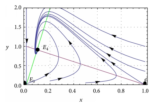
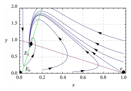
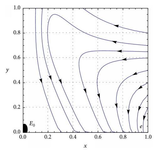
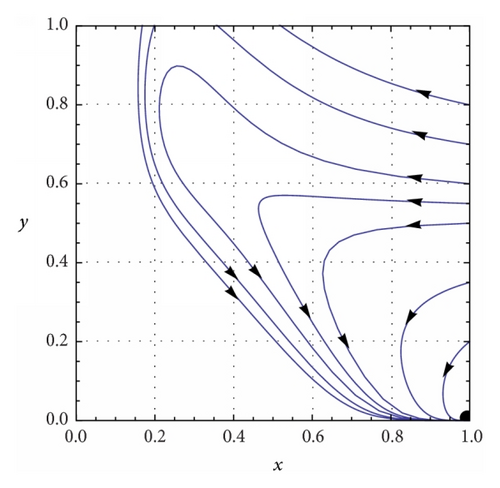
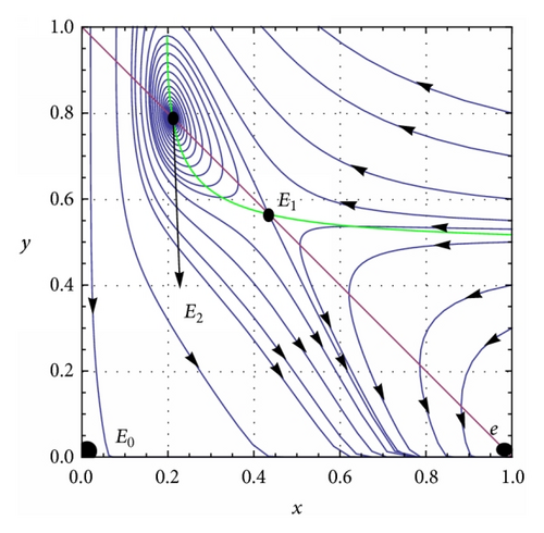
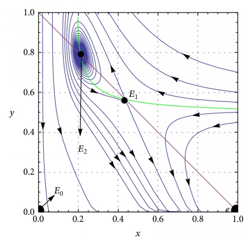
(a) β = 0.1, c = 0.01, and h = 0.5. System (5) has two interior equilibrium points E1 = (0.435558,0.564442) and E2 = (0.210806,0.789194), trivial equilibrium point E0 = (0,0), and an axial equilibrium point e = (1,0). If ρ = 0.75, the interior equilibrium point E2 is asymptotically stable (see Figure 2(a)) and if ρ = 0.9, the interior equilibrium point E2 is unstable (see Figure 2(b)). The axial equilibrium point e is an asymptotically stable point and the interior equilibrium point E1 is always a saddle point. If h = 0.01 and ρ = 0.9, system (5) has only one positive interior equilibrium point E4 = (0.091818,0.908182) which is globally asymptotically stable (see Figure 2(c)). If h = 0.05 and ρ = 0.9, system (5) has only one positive interior equilibrium point E5 = (0.0913611,0.908639) which is also globally asymptotically stable (see Figure 2(d)). β = 0.1, c = 0.01, and . System (5) has no positive interior equilibrium points and the phase portrait diagram is shown in Figure 2(e). The trivial equilibrium point is always a saddle.
Details are in the caption following the image
For ((a) and (b)) β = 0.1, c = 0.01, h = 0.5. (a) ρ = 0.75: the interior equilibrium point E2 = (0.210806,0.789194) is asymptotically stable, axial equilibrium point e = (1,0) is asymptotically stable, and interior equilibrium point E1 = (0.435558,0.564442) is a saddle point. (b) ρ = 0.9: the point E2 is unstable, e is asymptotically stable, and E1 is a saddle. (c) β = 0.1, c = 0.01, h = 0.01, and ρ = 0.9: the interior equilibrium point E4 = (0.091818,0.908182) is asymptotically stable; axial equilibrium point e = (1,0) is saddle. (d) β = 0.1, c = 0.01, h = 0.005, and ρ = 0.9: the interior equilibrium point E5 = (0.0913611,0.908639) is asymptotically stable; axial equilibrium point e = (1,0) is saddle. (e) The phase portrait diagram when no interior equilibrium exists. The origin is always a saddle.

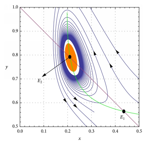
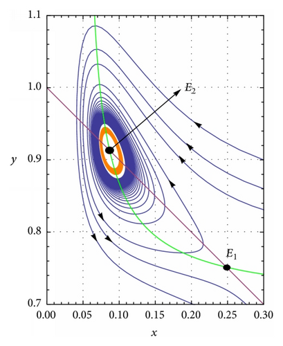
(b) β = 0.1, c = 0.01, h = 0.5, and then ρ = 0.865973. System (5) undergoes Hopf bifurcation and the first Lyapunov coefficient σ = 214.922 > 0, so an unstable limit cycle arises around the equilibrium point E2 = (0.210806,0.789194). Here, we take ρ = 0.854 (see Figure 3(a)). β = 0.02, c = 0.1, h = 0.8, and then ρ = 0.173169. System (5) undergoes Hopf bifurcation and the first Lyapunov coefficient σ = −762.219 < 0, so a stable limit cycle arises around the equilibrium point E2 = (0.0867959,0.913204). Here, we take ρ = 0.175 (see Figure 3(b)).
Details are in the caption following the image
(a) β = 0.1, c = 0.01, h = 0.5, ρ = 0.865973, and ρ = 0.854: an unstable limit cycle arises around the interior equilibrium point E2. (b) β = 0.02, c = 0.1, h = 0.8, ρ = 0.173169, and ρ = 0.175: a stable limit cycle arises around the interior equilibrium point E2.

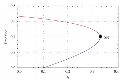
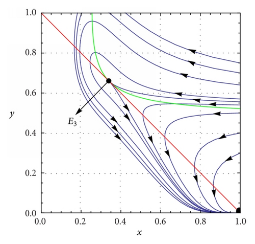
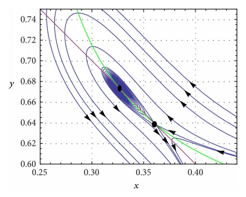
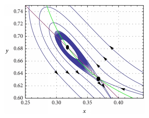
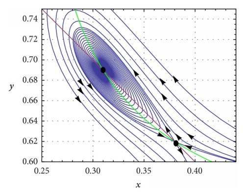
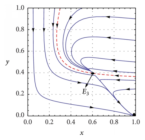
(c) β = 0.5, c = 0.1, ρ = 0.4, and . System (5) has a double interior equilibrium point which is a saddle node (see Figure 4(a)). The phase portrait diagram is shown in Figure 4(a) and the saddle-node bifurcation is shown in Figures 4(b) and 4(c).
Details are in the caption following the image
β = 0.5, c = 0.1, , and ρ = 0.4. System (5) has a double interior equilibrium point E3. (a) The point E3 is stable from above of the saperatrix curve and a saddle from below. ((b) and (c)) Saddle-node bifurcation diagram.
Details are in the caption following the image
β = 0.5, c = 0.1, , and ρ = 0.4. System (5) has a double interior equilibrium point E3. (a) The point E3 is stable from above of the saperatrix curve and a saddle from below. ((b) and (c)) Saddle-node bifurcation diagram.
Details are in the caption following the image
β = 0.5, c = 0.1, , and ρ = 0.4. System (5) has a double interior equilibrium point E3. (a) The point E3 is stable from above of the saperatrix curve and a saddle from below. ((b) and (c)) Saddle-node bifurcation diagram.
(d) β = 0.12 and c = 0.1; then, we obtain h0 = 0.583001 and ρ0 = 0.781849. Thus, system (5) is
()
System (40) has a unique positive interior equilibrium point E3 = (0.343303,0.656697).
Translating the equilibrium point E3 into the origin by using the transformations u1 = x − 0.343303 and u2 = y − 0.656697, by Taylor’s series expansion, system (40) reduces to
()
where α0(λ) = −0.678525λ2 − 0.867847λ1λ2, α1(λ) = 0.343303 + 0.439092λ1, α2(λ) = 0.343303 + 0.439092λ1 − 0.136546λ2 − 0.174645λ1λ2, α3(λ) = −1 − 1.27902λ1, α4(λ) = 1.04555 + 1.33727λ1, α5(λ) = −0.168089 − 0.214989λ1 + 0.18045λ2 + 0.230799λ1λ2, and R1(u1, u2) is a power series in (u1, u2) with powers satisfying i + j ≥ 3.
Making the affine transformations v1 = u1 and v2 = −0.343303u1 − 0.343303u2, then system (41) reduces to
()
where β0(λ) = 0.23294λ2 + 0.297935λ1λ2, β1(λ) = −0.0468767λ2 − 0.0599562λ1λ2, β2(λ) = 0.439092λ1 − 0.136546λ2 − 0.174645λ1λ2, β3(λ) = 0.759948 + 0.971988λ1 − 0.0619491λ2 − 0.0792341λ1λ2, β4(λ) = 0.381724 + 1.76725λ1 − 0.3609λ2 − 0.461599λ1λ2, and β5(λ) = 0.489622 + 0.626236λ1 − 0.525629λ2 − 0.67229λ1λ2.
Performing the C change of coordinates , w2 = v2β5v1v2 and z1 = w1, z2 = w2 + R3(w1, w2) in the small neighbourhood of (0,0), system (42) reduces to
()
where γ0(λ) = 0.23294λ2 + 0.297935λ1λ2, , γ2(λ) = 0.439092λ1 − 0.136546λ2 − 0.174645λ1λ2, γ3(λ) = 0.759948 + 0.971988λ1 − 0.273381λ2, γ4(λ) = 0.381724 + 1.76725λ1 − 0.3609λ2 − 0.461599λ1λ2, and F1, F2, and F3 are the power series in z1 and (z1, z2) with powers , and satisfying k1 ≥ 3, k2 ≥ 2, and i + j ≥ 1, respectively.
Applying the Malgrange Preparation theorem, we have
()
where B(0, λ) = γ3 and B is a power series in z1 whose coefficients depend on parameters (λ1, λ2).
We have γ3 = 0.759948 > 0 as λ1, λ2 → 0. We take the transformation
()
then, system (43) reduces to
()
where S1(X1, X2, 0) is a power series in (X1, X2) with powers satisfying i + j ≥ 3 and j ≥ 2.
Applying the parameter dependent affine transformations Y1 = X1 + γ1/2γ3 and Y2 = X2 in system (46), we obtain
()
where S2(Y1, Y2, 0) is a power series in (Y1, Y2) with powers satisfying i + j ≥ 3 and j ≥ 2.
Consider the C transformation
()
Then, system (47) reduces to
()
where , , and S3(X, Y, 0) is a power series in (X, Y) with powers XiYj satisfying i + j ≥ 3 and j ≥ 2. Also . Thus, system (40) undergoes Bogdanov-Takens bifurcation.
The local representations of the bifurcation curves are as follows:
  • (a)

    SN = {(λ1, λ2) : μ1(λ1, λ2) = 0,   μ2(λ1, λ2) ≠ 0}.

  • (b)

  • (c)

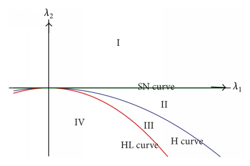
These bifurcation curves are sketched in a small neighbourhood of the origin in the λ1λ2 plane (see Figure 5(a)). The bifurcation curves divide the parameter plane into four parts: I, II, III, and IV. The saddle-node bifurcation curve (SN) is the horizontal axis, that is, λ2 = 0 axis, and the homoclinic bifurcation curve (HL) and Hopf bifurcation curve (H) lie in the fourth quadrant. When (λ1, λ2) = (0,0), then system (5) has a unique interior equilibrium point which is a cusp of codimension 2 (see Figure 5(b)). When the parameters λ1 and λ2 vary and lie in region I, then system (5) has no interior equilibrium point and all the solution trajectories go to the axial equilibrium point; that is, the axial equilibrium point is globally stable (see Figure 5(c)). Hence, in this case, the predator will go extinct and prey will approach the carrying capacity. When the parameters λ1 and λ2 pass the SN bifurcation curve and lie in region II, the cusp of codimension 2 breaks into a hyperbolic saddle and an unstable focus (see Figure 5(d)). When the parameters λ1 and λ2 lie in region III, the cusp of codimension 2 breaks into a stable focus and a hyperbolic saddle. The change of stability of the focus yields an unstable limit cycle (see Figure 5(e)). Further, when the parameters λ1 and λ2 lie in region IV, the cusp of codimension 2 breaks into a saddle point and a stable focus (see Figure 5(f)). Hence, an open set of initial population densities exists for which both predator and prey approach a stable steady state.
Details are in the caption following the image
β = 0.12, c = 0.1, h0 = 0.583001, and ρ0 = 0.781849. (a) BT bifurcation diagram in the λ1λ2 plane. (b) The equilibrium point E3 is a cusp when (λ1, λ2) = (0,0). (c) No interior equilibrium point exists when (λ1, λ2) = (0.04,0.001) lies in region I. (d) An unstable focus when (λ1, λ2) = (0.03, −0.001) lies in region II. (e) An unstable limit cycle when (λ1, λ2) = (0.03, −0.002) lies in region III. (f) A stable focus when (λ1, λ2) = (0.03, −0.004) lies in region IV.

6. Discussion and Conclusion

In this paper, a Leslie-Gower predator-prey model has been analyzed in the presence of nonlinear predator harvesting. It is shown that the system has at most four equilibrium points in Ω, in which the trivial equilibrium point and the axial equilibrium point always exist while the positive interior equilibrium point changes from two to zero. The qualitative properties of solutions in the vicinity of (0,0) have been studied by using a blow-up technique, and it is found that the origin will never be stable; ecologically speaking, the two species cannot go to extinction together. The axial equilibrium point is either asymptotically stable or globally stable or a saddle depends on the parametric conditions. Thus, ecologically speaking, the prey species never goes to extinction whatever the choice of initial population density. If two interior equilibrium points exist, then one is always a saddle point while the other is either asymptotically stable or unstable or the system undergoes a Hopf bifurcation around this point; that is, for certain parametric domain, the system exhibits a bistability phenomenon as well as oscillatory coexistence of both the populations. The stability of limit cycles has been studied and validated through numerical simulations by calculating the first Lyapunov number. It is also found that for certain parametric domain the proposed system has a unique interior equilibrium which is globally asymptotically stable.

It is shown that the system can have zero, one, or two interior equilibrium points through saddle-node bifurcation as the bifurcation parameter h crosses a certain threshold value. By means of Sotomayor’s theorem, the existence of saddle-node bifurcation has been shown. Ecologically speaking, a maximum threshold value of h exists, below which both species coexist and above which predator species suddenly collapse to extinction. The proposed system undergoes Bogdanov-Takens bifurcation near degenerate equilibria. We have considered the parameters h and ρ as bifurcation parameters and reduced the system into normal form. Ecologically speaking, a small perturbation in the bifurcation parameters is a cause of extinction, coexistence, and oscillation.

The dynamical analysis of model (5) shows complex and rich dynamics as compared to the model with no harvesting [21] and with constant-yield predator harvesting [19]. The model without harvesting has a unique interior equilibrium point which is globally asymptotically stable [21] while model (5) has zero to two interior equilibrium points and model (5) undergoes a series of bifurcations (Hopf bifurcation, saddle-node bifurcation, and Bogdanov-Takens bifurcation). The model with constant-yield predator harvesting has no axial equilibrium point, and the solutions once touching the x-axis will leave the first quadrant [21]. But the model with nonlinear predator harvesting has one trivial equilibrium point E0 = (0,0) and one axial equilibrium point e = (1,0) and the solutions touching the x-axis will go to the axial equilibrium point e. Further, if no interior equilibrium point exists, then the axial equilibrium point e is globally asymptotically stable (see Figure 2(e)). Ecologically speaking, in the absence of predator species, the prey density approaches the carrying capacity. Although the model with constant-yield predator harvesting undergoes a series of bifurcations, like Hopf bifurcation, saddle-node bifurcation, and Bogdanov-Takens bifurcation [19], the model with nonlinear harvesting gives more general parametric conditions for the occurrence of these bifurcations. Thus, the results of nonlinear harvesting model can explain the real life situation in a more effective and realistic manner.

Competing Interests

The authors declare that they have no competing interests.

    The full text of this article hosted at iucr.org is unavailable due to technical difficulties.