Diffusion Filters for Variational Data Assimilation of Sea Surface Temperature in an Intermediate Climate Model
Abstract
Sequential, adaptive, and gradient diffusion filters are implemented into spatial multiscale three-dimensional variational data assimilation (3DVAR) as alternative schemes to model background error covariance matrix for the commonly used correction scale method, recursive filter method, and sequential 3DVAR. The gradient diffusion filter (GDF) is verified by a two-dimensional sea surface temperature (SST) assimilation experiment. Compared to the existing DF, the new GDF scheme shows a superior performance in the assimilation experiment due to its success in extracting the spatial multiscale information. The GDF can retrieve successfully the longwave information over the whole analysis domain and the shortwave information over data-dense regions. After that, a perfect twin data assimilation experiment framework is designed to study the effect of the GDF on the state estimation based on an intermediate coupled model. In this framework, the assimilation model is subject to “biased” initial fields from the “truth” model. While the GDF reduces the model bias in general, it can enhance the accuracy of the state estimation in the region that the observations are removed, especially in the South Ocean. In addition, the higher forecast skill can be obtained through the better initial state fields produced by the GDF.
1. Introduction
An outstanding issue of either CSM or RFM is its inefficiency in capturing the spatial multiscale information by observations. A difficulty in practice is how to properly choose the characteristic length scales Lx and Ly in the CSM or the filter coefficient α in the RFM. Observational studies show that (Lx, Ly) change with location, depth, and time [14–16]. If they are too large, the analysis is too smooth and shortwave information is lost. If they are too small, the analysis lacks coherent structure in data sparse regions because the longwave information cannot be properly corrected. Thus, in the past it has been thought that the characteristic length scales (Lx, Ly) in the CSM or the filter coefficient α in the RFM is responsible for the unsatisfactory analysis in the 3DVAR.
To avoid empirically or statistically setting the characteristic length scales and to correctly minimize the longwave and shortwave errors in turn, a sequential 3DVAR (S3DVar) method was developed [17] to assimilate sea surface temperature (SST) in a global ocean model [18]. The S3DVar method is simply composed of a series of 3DVars, each of which uses recursive filters with different filter coefficients. These 3DVars sweep through all resolvable scales by observational networks from longwaves to shortwaves. In addition, a multigrid data assimilation scheme was also introduced to extract the resolvable information from longwave to shortwave in an observational system [19]. Recently, a sequential variational approach based on the multigrid data assimilation method was proposed to accurately retrieve the multiscale information from available observation systems [20].
Since the matrix B is treated as the Gaussian type in the CSM and modeled as the diffusion process (or Gaussian filtering process) in the RFM, the spread of the information from the analysis point to the entire region is interpreted as the diffusion phenomenon [21]. The diffusion filter (DF) was developed on the base of the Gaussian diffusion process and therefore can be used directly to model B. Several spatial multiscale variational analysis schemes, based on the modification to the standard DF scheme, are proposed in this study. As a pilot study, one of the spatial multiscale variational analysis schemes, the gradient DF (GDF), is used to assimilate SST observations into an intermediate coupled model within a perfect “twin” experiment framework.
The paper is organized as follows. The methodology of the standard DF scheme is described in Section 2. Several spatial multiscale DF schemes are presented in Section 3. In Sections 4 and 5, simple observing/assimilation system simulation experiments and global SST simulation with an intermediate coupled atmosphere-ocean-land model are conducted to evaluate one of the new DF schemes, that is, the gradient DF (GDF), on the model estimation and forecast. The conclusions are summarized in Section 6.
2. Diffusion Filter
- (1)
Choose an appropriate diffusion coefficient a; give the initial guess of w (w = 0, for instance).
- (2)
Integrate the diffusion model (9) from “time” t = 0 to S to obtain uS(w).
- (3)
Calculate f according to (12).
- (4)
Integrate the adjoint model (11) from “time” t = S to 0 to obtain R0(w); then the gradient g(w) of the cost function J is −R0(w).
- (5)
Use descent algorithms to adjust w.
- (6)
Loop from step (2) until the convergence criterion is met.
Use of DF for determining the matrix B is called the DF method (DFM), which has the same computation loads as the RFM if the ADI difference scheme (or the other operator splitting scheme; see Appendix) is applied to calculate the diffusion equation (9). The diffusion filter scheme has the same problem as the recursive filter scheme in extracting observational information. As the extent of spatial dispersion is only determined by diffusion coefficient a when “time” duration t is set to be constant, if a is large, the shortwave information will be lost. Conversely, if a is small, the longwave information will not be properly captured. Obviously, the diffusion coefficient a plays the same role as the filter coefficient α does in the recursive filter scheme.
3. Spatial Multiscale Diffusion Filters
To retrieve longwave information over the whole domain and shortwave information over data-dense regions, three spatial multiscale variational analysis schemes, based on the diffusion filter, are proposed.
3.1. Sequential Diffusion Filter (SDF)
The sequential diffusion filter (SDF) scheme is similar to the S3DVar method derived by Xie et al. [17]. The SDF scheme uses a sequence of 3DVars to obtain the final estimation to retrieve information from all wavelengths from long- to shortwaves in turn. The matrix B is modeled by applying the diffusion filter sequentially in x and y direction, respectively. SDF begins its sequence with a big value of the diffusion coefficient a; then an initial estimation is obtained through analyzing the observed data. After that, a S3DVar is solved using the diffusion filter with a smaller a than before. For the S3DVars, observations to be assimilated are produced by subtracting the previously analyzed values from the observations assimilated by the previous 3DVar until the diffusion coefficient a is small enough. The final estimation is the summation of all the previous 3Dvar analyses based on the diffusion filter.
From the above description, it is noted that the SDF scheme is a simple extension of the DF, in which information is retrieved step by step from long- to shortwaves. During the process of the SDF, B is changed gradually with the different diffusion coefficient a and thus becomes flow dependent and anisotropic following the multiscale information of the observation.
3.2. Adaptive Diffusion Filter (ADF)
Due to the introduction of the heat diffusion equation, the gradient of the cost function with respect to the state variables can be obtained using the adjoint method with 4DVar. In general, the diffusion coefficients a(x, y) and b(x, y) are not constants but are space dependent. Therefore, it is possible to optimize not only the state variables but also the diffusion coefficients using 4DVar. State variables and diffusion coefficients are used together as control variables, so values of a(x, y) and b(x, y) will change adaptively according to the distribution of observations.
3.3. Gradient Diffusion Filter (GDF)
The algorithm is a variant of the spatial multiscale recursive filter [22]. For small diffusion coefficients a, b, the gradient contains not only all the observational signals from longer to shorter wavelengths, but also a lot of erroneous signals in data sparse regions, which causes lack of coherent longwave structure in space. If this gradient is simply introduced into the minimization algorithm without careful considerations, the analysis departs far from reality. Thus, a prerequisite for the minimization algorithm used in 3DVAR is needed to extract the longwave information from the gradient and at the same time to preserve the valuable shortwave signals.
However, the longwave information implied in the gradient cannot be made best use of to construct a reasonable descent direction in general minimization algorithms. Take the steepest descent algorithm as an example, in which the descent direction is simply chosen as −g(w). Suppose the initial guess of w (i.e., w0) is equal to zero. Then at the ith iteration, the new solution wi = wi−1 + li−1∗(−g(wi−1)) is obtained by using a line search algorithm to find an appropriate step size li−1. According to what have been indicated, the gradient g(w0) actually represents certain scales of observations d, and these scales will be extracted by the line search at the first iteration and incorporated into a new solution w1. However, if the diffusion coefficients a, b are small, the gradient g(w0) will lack coherent structure in data sparse regions though it actually carries all observational signals. And since the new solution w1 is simply obtained along the descent direction, −g(w0), the same problem will also exist in w1, which indicates that the longwave information of observations d is not effectively extracted from the gradient g(w0) at the first iteration. Similarly, at the second iteration, the longwave information of the observation residue after the first iteration will not be extracted from the gradient g(w1) and incorporated into the new solution w2, and so on. As a consequence, in data sparse regions, the final analysis will also lose the longwave structure of observations. The same problem also exists for other minimization algorithms such as BFGS and the conjugate gradient method, for the same reason.
- (1)
Give an initial guess of w (i.e., w0) which equals zero. Then select diffusion coefficients a, b as small ones and give a large enough value to an extra diffusion coefficient denoted as β.
- (2)
Use the diffusion filter with coefficient a, b to calculate Bw in (5).
- (3)
Calculate the difference between observations d and HBw, namely, the observation residue.
- (4)
Calculate the gradient g of the cost function J with respect to w using the DF through the adjoint model.
- (5)
Apply the diffusion filter with coefficient β on −g to calculate the descent direction E(−g), where E represents a positive definite operator.
- (6)
Select E(−g) as the descent direction, and use line search algorithm to find the step size, l; then w is adjusted to w = w + l∗E(−g).
- (7)
The value of β diminishes.
- (8)
Loop from step (2) until the convergence criterion is met.
If the background term Jb is involved in the cost function J, the same procedure is performed except that g calculated in step (4) is the gradient of cost function J, which includes both Jb and Jo.
4. Observing/Assimilation System Simulation Experiments
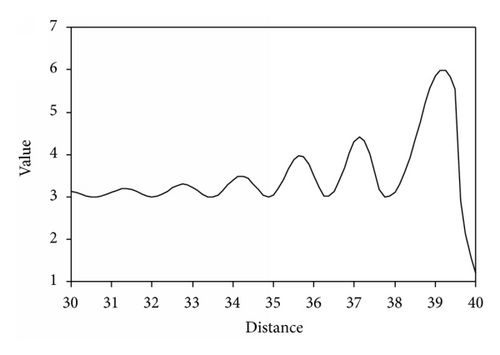
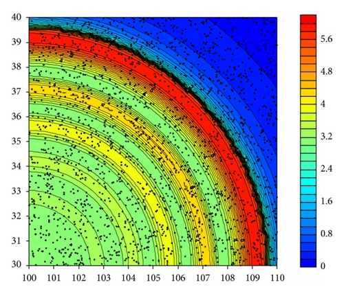
Observing/assimilation system simulation experiments are performed to evaluate the spatial multiscale variational analysis. The “truth” field in these experiments is represented by an analytic temperature field defined over the area of 100°E–110°E and 30°N–40°N. The “truth” field of the temperature is plotted in Figure 1(b), whose high nonlinearity can be seen from Figure 1(a). The grid resolution is set to 1/8° × 1/8°, and the total numbers of the grid are 80 × 80. The observational dataset is generated using the analytic solution. Observational error is simulated by adding a sample of white noise with a standard deviation of 0.2 to the “truth.” Three experiments are conducted in which different configurations of numbers of observations are employed.
4.1. Experiment 1
In this experiment, the number of observations is set to 2000 at first, and the observations are randomly and uniformly distributed in the whole domain, which can be seen from the black dots in Figure 1(b). In the experiment with DF, several values of the diffusion coefficient are used to verify the impacts on the analyzed field. In the experiment with GDF, the processes (1)–(8) described in Section 3.3 are conducted. The diffusion coefficients a, b are set to a small value, of 0.1, which suggests almost all the observational signals, from long to short wavelengths, can be retrieved. However, a large enough value, 1.0, is given to the extra diffusion coefficient β of the gradient at the first step. For the subsequent steps, β is reduced by 0.1 from the previous step. At the last step, β becomes 0.1, which is small enough for the case. The limited memory BFGS quasi-Newton minimization algorithm [23] is used during the minimizing procedure.
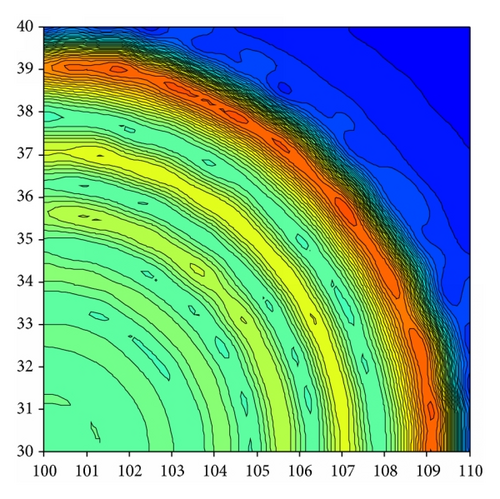
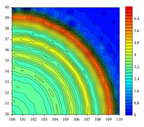
The major scales of the truth field are reconstructed by 2000 observations almost fully using the GDF (Figure 2(a)), but not well reconstructed using the DF with different diffusion coefficients (a, b): 1.0 (Figure 2(b)), 0.5 (Figure 2(c)), and 0.1 (Figure 2(d)). The small scale features begin to dominate the analyzed fields when the diffusion coefficients are reduced gradually, while the large scale signals are contaminated dramatically by an abundance of small scale features.
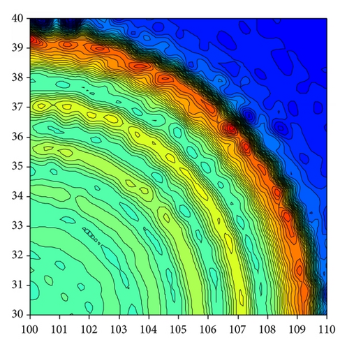
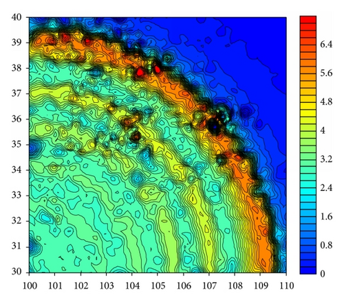
As He et al. [18] indicated, artificial signals can be produced during the data assimilation if the chosen diffusion coefficient cannot represent the actual scale. In contrast, the GDF can handle spatial multiscale analysis pretty well compared to the simple DF with a fixed diffusion coefficient. In addition, the GDF is easy to avoid in empirical selection of the diffusion coefficient.
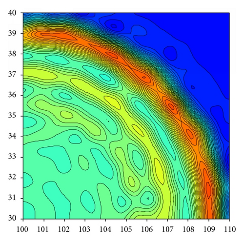
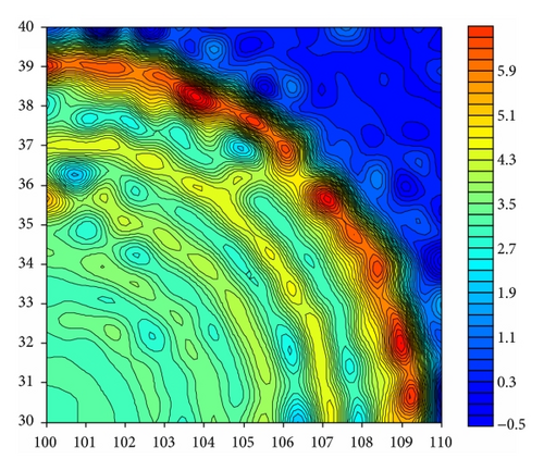
Figure 3 shows the performance of GDF and DF when the number of observations decreases from 2000 to 500. The GDF (Figure 3(a)) can retrieve large scale information from observations and leave the unresolved scale as errors on top of the resolvable scales. These errors are smaller than those generated by DF with a fixed diffusion coefficient (Figure 3(b)) in the condition of the sparseness of the observations and the lack of information.
4.2. Experiment 2
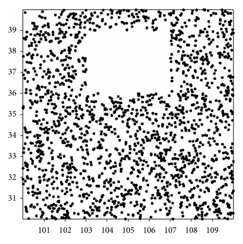
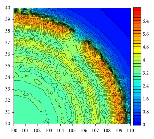
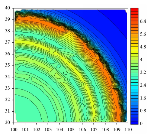
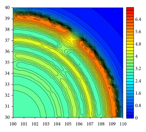
The second experiment is conducted with removal of observations in the area of 103°E~107°E and 35°N~40°N (Figure 4) to further evaluate the GDF capability in retrieving the multiscale information from observations. The analyzed field of the GDF (Figure 5(a)) performs much better in the data void region than that of the DF with (a, b) = 0.8 (Figure 5(b)) and 0.5 (Figure 5(c)). The GDF can reconstruct the temperature field (Figure 5(a)) reasonably well despite the absence of the observations in the region as shown in Figure 4. The spatial pattern of the whole temperature field can be captured roughly according to the large scale information derived from all the observations in the whole analyzed region. However, the DF fails to reconstruct the temperature field and produces false features especially in the data void region. For example, a strong cold tongue is produced for (a, b) = 0.8 (Figure 5(b)), and large scale temperature field is distorted with displacement of the thermal front in the data void region for (a, b) = 0.5 (Figure 5(c)). Little information of the observations can be extracted from data rich area to the data void region using DF.
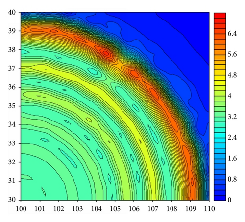
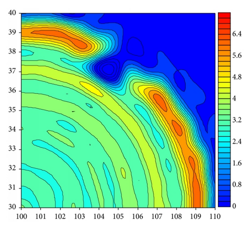
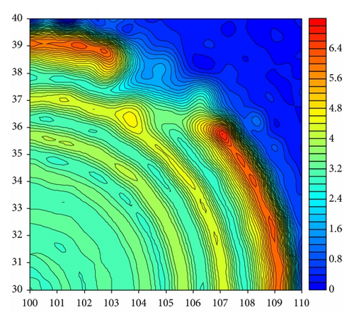
Such capabilities make the GDF invaluable to get well represented values for the data void (or insufficiently covered) areas such as a typhoon-affected area during typhoon passage or the Southern Hemisphere Oceans (compared to other ocean basins). The GDF can reconstruct the analyzed field roughly according to the longwave information of the observations beyond the data void area such as typhoon-affected region or the Southern Ocean. On the other hand, both the standard DF and the traditional RF may lead to false results in the data void region, as shown in Figures 5(b)-5(c); an improper analysis is also likely to be produced, which will affect the analysis/forecast accuracy seriously.
In addition, several classical geostatistical tools, such as inverse distance to a power, triangulation with linear interpolation, and Kriging method are used to interpolate such observations (no white noise is imposed on the observations). Compared to the other two geostatistical tools, the Kriging method is able to accurately fill in the hidden information (Figures 6(a) and 6(b) versus 6(c)). However, compared with the variational method, the geostatistical tools have a limited application and cannot handle corrections between different analysis variables or physical balances and other constraints [20].
5. Global SST Assimilation Using GDF
In this section, we apply the GDF to assimilate the SST into an intermediate climate model to improve the climate representation and forecast.
5.1. Brief Description of an Intermediate Atmosphere-Ocean-Land Coupled Model
All the three model components adopt 64 × 54 Gaussian grid and are forwarded by a leap frog time stepping with a half hour integration step size. There are 2287 and 1169 grid points over the ocean and land, respectively. An Asselin-Robert time filter [30, 31] is introduced to damp spurious computational modes in the leap frog time integration. Default values of all parameters are listed in Table 1 in Wu et al. [24].
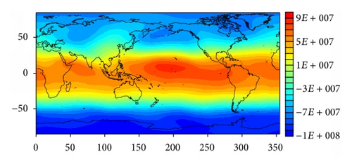
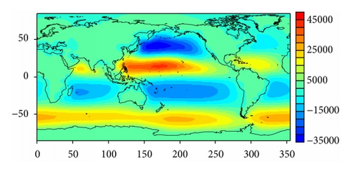
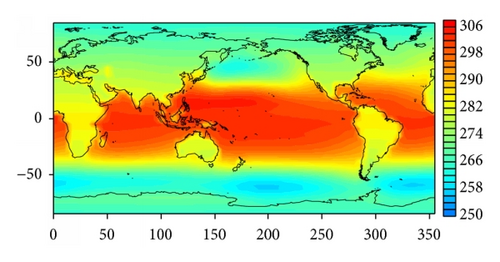
Starting from initial conditions , where ψ0, ϕ0, , and are zonal mean values of corresponding climatological fields, the coupled model is run for 60 years to generate the model states ). The last 10 years’ model states (Z1) are used as the “truth” fields. Figure 7 shows the annual mean of ψ (Figure 7(a)), ϕ (Figure 7(b)), To and Tl (Figure 7(c)), where the associated wave trains in the ψ field are observed. For ϕ, one can see the distinct pattern of the western boundary currents, gyre systems and the Antarctic Circumpolar Current (ACC). For To and Tl, reasonable temperature gradients are also produced. Note that the low temperature in tropical lands can be attributed to the linear damping of KT in the solar forcing. The above model configuration is called the “truth” model, which has reasonable but rough representation for the basic climate characteristics of the atmosphere, land, and ocean.
5.2. Model “Bias” Arising from the Initial States
However, starting also from the same initial conditions Z0, the Gaussian random numbers are added to ψ0 and ϕ0, with standard deviations of 107 m2s−1 (for ψ0) and 105 m2s−1 (for ϕ0), respectively. The coupled model is also run for 60 years to generate the model states . The last 10 years’ model states are used for analysis. This model configuration is called the biased model.
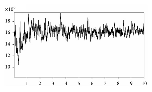
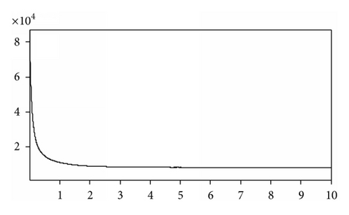
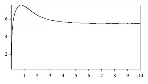
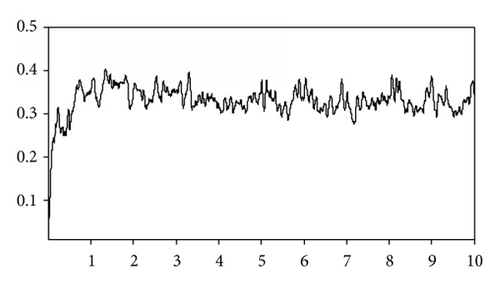
The model “biases” induced by perturbed initial fields are examined. Figure 8 shows time series of the spatial averaged root mean square errors (RMSEs) of ψ, ϕ, To, and Tl for the assimilation model, which are calculated according to the difference in the assimilation model and the “truth” model. The obvious difference about all the four components can be seen from Figure 8. The RMSE of ψ reaches about 1.6 × 10⁷ m2s−1 with a high frequent oscillation (see Figure 8(a)). In contrast, the RMSE of ϕ performs smoothly and rapidly decreases within the first year and gradually reaches a low and stable value about 104 m2s−1 (see Figure 8(b)). The RMSEs of To (Figure 8(c)) and Tl (Figure 8(d)) increase rapidly in the first year, which are generated by the initially perturbed ψ0 and ϕ0 through the coupling. High frequency oscillation is noted in the time series of the RMSE of Tl, which indicates that the land surface temperature Tl is dominated by the atmospheric motion (ψ). However, time series of the RMSE of To is much smoother than that of Tl, indicating that To is modulated by the oceanic motion (ϕ).
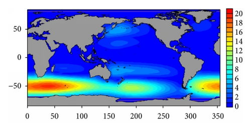
The spatial distribution of RMSE of To for the biased model (Figure 9) shows a notable bias in the ACC region of the Southern Ocean with a maximum value over 15 K near the southern tip of Africa. Besides, obvious biases also exist in the west boundaries of the ocean in the subtropical regions.
5.3. Twin Experiment Design
In this section, with the intermediate model and DF/GDF data assimilation scheme described above, a perfect twin experiment framework is designed with the assumption that the errors of initial model states are the only source of assimilation model biases. Starting from the model states, Z1, described in Section 5.1, the “truth” model is run for 1 year to generate the time series of the “truth” states. Only synthetic observations of To are produced through sampling the “truth” states at specific observational frequencies. A Gaussian white noise is added for simulating observational errors. The standard deviations of observational errors are 0.5°C for To. The sampling period is 24 hours. The “observation” locations of To are global randomly distributed with the same density of the ocean model grid points.
The biased model uses the biased initial fields depicted in Section 5.2. Starting from the biased model states, Z2, the experiment E_GDF consists on assimilating observations into model states using the GDF scheme. In comparison, the experiment E_DF is carried out, where the standard DF scheme is used with the diffusion coefficients a, b = 0.5. In addition, a control run without any observational constraint, called CTRL, serves as a reference for the evaluation of assimilation experiments.
5.4. Impact of the GDF on the Estimate of the States
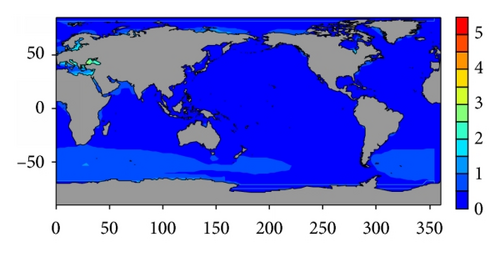
The performance of GDF is investigated. Figures 10(a)–10(d) show time series of RMSEs of ψ, ϕ, To, and Tl for the CTRL (solid line) and the GDF (dash line). Compared to the CTRL (solid line in Figure 10(c)), To of the GDF has significant improvement (dash line in Figure 10(c)), in which the RMSE decreases to approximately 0.5 K. Figure 11 presents the spatial distributions of RMSEs of To using GDF. The RMSE of To over ocean is obviously reduced compared with that of the CTRL (see Figure 9), especially in the Southern Ocean, the subtropical and the subpolar regions. In particular, the reduction of RMSE is much significant in the ACC region, in which the RMSE decreases from above 15 K to below 3 K.
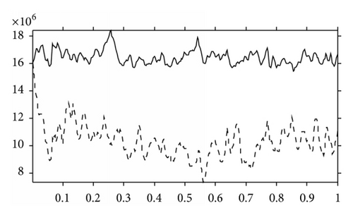
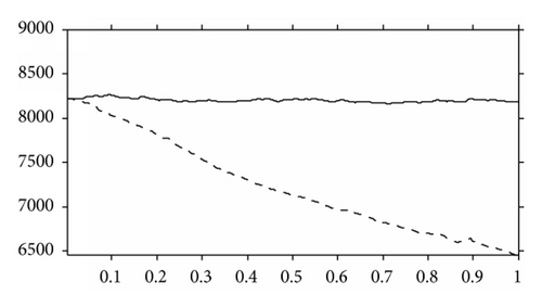
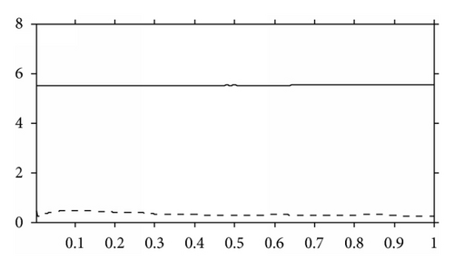
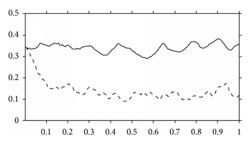
Unlike the RMSEs of To, there is no direct observations constraint for ψ, ϕ, and Tl; therefore, their RMSEs decrease gradually owing to the effect of the coupling. The RMSEs of ψ for the GDF are reduced significantly from about 1.6 × 10⁷ m2s−1 to about 1.1 × 10⁷ m2s−1 with a high frequent oscillation (see Figure 10(a)). The ϕ in GDF is also improved significantly comparing to CTRL (solid versus dash lines in Figure 10(b)), whose RMSE decreases gradually and smoothly, but it does not reach a stable value within the experimental period, indicating that the low frequency signal needs a much longer time to reach equilibrium compared to the high frequency signal. For Tl, the GDF reduces the error by approximately 60%. Note that To has no direct effect on Tl, which can be realized according to the framework of the coupling model (see (18)–(20)). Instead, To affects Tl indirectly via ψ. The improved To by the observational constraint increases the quality of ψ over land through the dynamical constraint. Then, the improved ψ ameliorates Tl through the process of the external forcing.
5.5. Removal of Observational Data in the Southern Ocean
In the real ocean, the observations are scarce in the southern polar region. Therefore, another set of data assimilation experiment is carried out, which is the same as the experiment in Section 5.3, but in which the observations, south of 50°S and 50°E~300°E, are removed completely.
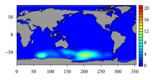
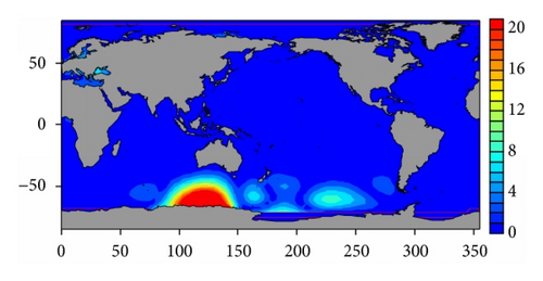
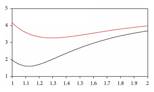
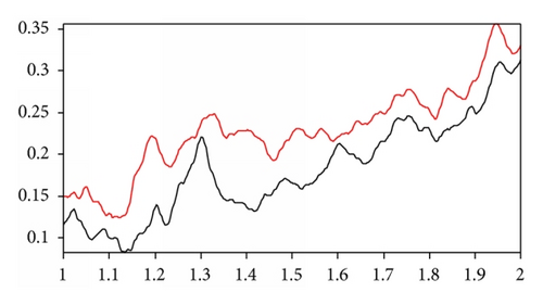
Figures 12(a)–12(d) show the time series of RMSEs of ψ, ϕ, To, and Tl with the GDF (black line) and the standard DF with a, b = 0.5 (red line). The RMSE of To for the DF increases persistently during the experimental period, while the RMSE for the GDF begins to descend after 0.2 years and converges after 0.6 years (Figure 12(c)). When the diffusion coefficients are set to different values in the DF experiment (e.g., a, b = 0.2,0.8,1.0), similar results as the ones presented in Figure 12 are obtained. Results indicate that DF cannot correct the model bias in the data void region. However, the GDF is able to mitigate the model bias to some degree through extracting the spatial multiscale information from the available observations to the data void region. Figure 13 presents the spatial distributions of RMSEs of To for the GDF and the standard DF with a, b = 0.5. Compared to the DF, the GDF produces a significant improvement within the data void region in the Southern Ocean (compare Figures 13(a) and 13(b)).
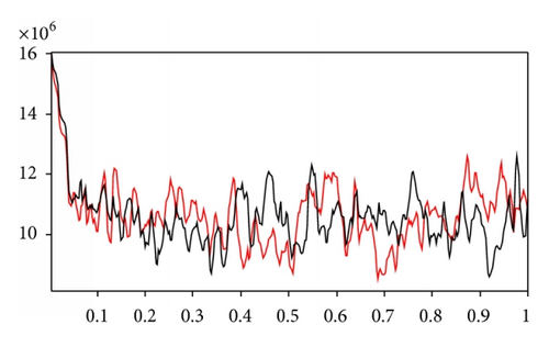
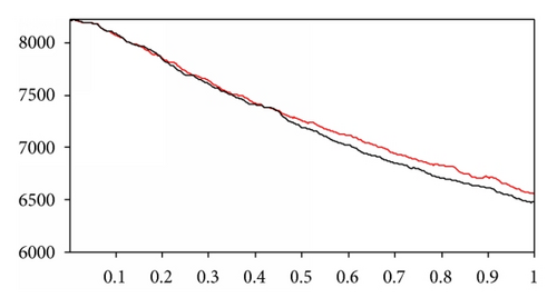
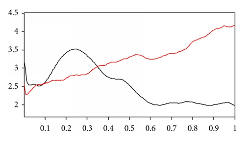
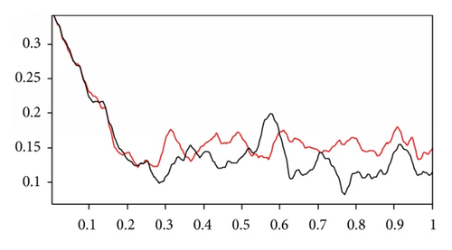
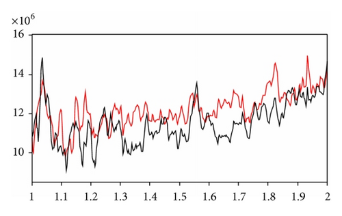
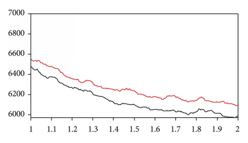
The RMSE of ψ in the GDF is not always smaller than the DF owing to the strong nonlinear nature of the high frequent atmosphere (red line versus black line in Figure 12(a)). In contrast, the evolution of Tl in the model (see (20)) is rather simple (i.e., linear); the RMSE in the GDF is almost always smaller than that for the DF (red line versus black line in Figure 12(d)). For the low frequent component ϕ (see Figure 12(b)), the RMSEs of both the GDF and the DF decrease gradually, indicating that the effect of the data void region on the low frequent signal is small in the given time scale.
5.6. Impact of the GDF on the Forecast
From a more practical point of view, the role of the GDF should be judged from the model forecast. In this section, two forecast experiments without any observational constraint are integrated for 1 year, respectively, starting from the final analyzed states of the above two assimilation experiments (the GDF and the DF).
Figures 14(a)–14(d) show the forecasted time series of RMSEs of ψ, ϕ, To, and Tl for the GDF (black line) and the DF with a, b = 0.5 (red line). The GDF performs much better than the DF in 1 year’s forecast lead time of all the state variables such as the high frequent component ψ and the low frequent component ϕ (black versus red curves in Figures 14(a) and 14(b)). It is interesting that the forecasted RMSE of ϕ still decreases inertially owing to the longer adjustment time of the low frequent signal, but whose trend becomes mildly with the increase of the forecasted lead time. For To, because of the absence of the observational constraint, the forecasted RMSE has an obvious positive trend (see Figure 14(c)), indicating that the forecasted state is gradually drifting away from the truth. Anyway, the GDF retains its superiority relative to the DF during the entire forecasted lead time. The forecasted RMSEs of Tl have similar patterns to those of To (see Figure 14(d)).
6. Conclusions and Discussions
In this study, the diffusion filter (DF) is introduced as a concrete implementation of the 3DVAR scheme. Similar to the recursive filter (RF), the outstanding issue of DF is its inefficiency in capturing the spatial multiscale information resolved by observations. Therefore, several spatial multiscale variational analysis schemes based on the DF are proposed to retrieve the spatial multiscale information from longwaves to shortwaves. As one of the spatial multiscale variational analysis schemes, the gradient diffusion filter (GDF) scheme is proposed and verified through a set of observing/assimilation system simulation experiments, where the “truth” field of the sea surface temperature is represented by a high nonlinear analytic function in a given sea region, and the observations are sampled randomly and uniformly in the whole domain. Results of the assimilation experiments indicate that the GDF has noticeable advantages over the standard RF and DF schemes, especially in the data void region. The GDF can retrieve the longwave information over the whole domain and the shortwave information over data-dense regions.
After that, a perfect twin experiment framework is designed to study the effect of the GDF on the state estimation based on an intermediate atmosphere-ocean-land coupled model. In this framework, the assimilation model is subject to “biased” initial fields from the “truth” model. The RMSE of the sea surface temperature can be reduced significantly through the observational constraint via the GDF. At the same time, the RMSEs of the other model components, such as the land surface temperature and the atmospheric and oceanic stream functions can also be mitigated by the dynamical constraint and the external constraint through the ocean-atmosphere-land coupled process. For simulating the real observational networks in the world ocean roughly, the observations locating in the Southern Ocean are removed to investigate the role of the GDF in retrieving the multiscale information from observations. While the standard DF hardly removes the model bias in the data void region, the GDF may mitigate the model bias to some degree through extracting the multiscale information from the observations beyond the data void region. In addition, the higher forecast skill can also be obtained through the better initial state fields produced by the GDF.
It should be noted that the background term Jb is omitted in the above assimilation experiments. When high-density, accurate, resolvable information is available in observational datasets, it is much essential to extract the multiscale information from the observations with deterministic data assimilation approaches, as this study does. High-quality background fields can be obtained firstly when deterministic data assimilation approaches are carried out. Next, the statistical data assimilation approaches, such as traditional 3DVar and 4Dvar, can be used to treat observations as random variables, in which Jb will be included to extract the information that cannot be resolved by the observation networks.
In spite of the promising results produced by the GDF in the intermediate climate model, much work is needed to explore the impact of the multiscale variational analysis schemes on the state estimation and forecast in real applications using general circulation models (GCMs). In addition, other spatial multiscale variational analysis schemes based on the DF, such as the adaptive diffusion filter (ADF) scheme, should also be studied to further improve the convergence speed and accuracy.
Conflict of Interests
The authors declare that there is no conflict of interests regarding the publication of this paper.
Acknowledgments
The authors would like to express their gratitude to two reviewers for their helpful comments and suggestions, which contributed to greatly improve the original paper. This work was supported by the National Basic Research Program of China (no. 2013CB430304), National High-Tech R&D Program of China (no. 2013AA09A505), and National Natural Science Foundation of China (nos. 41206178, 41376015, 41376013, and 51379049).


